1.6 Linkage disequilibrium

Every human genome has a unique DNA sequence, in part due to the few hundred novel mutations inherited from their parents, and by chromosomal segregation combined with crossovers that shuffle existing variation. However, although every human genome may be unique, certain combination of variants (e.g. SNP) may be shared by few individuals and sometimes by a large fraction of the population, resulting in allelic association also known as haplotype structure. The term linkage disequilibrium (LD) is broadly used to refer to the non-random association of combination of variants, therefore LD neither requires genetic linkage nor is particularly a disequilibrium.

Particular alleles at neighbouring loci tend to be co-inherited. For tightly linked loci, this might lead to associations between alleles in the population resulting in high LD between these loci. LD has recently become the focus of intense study in the hope that it might facilitate the mapping of complex disease loci through whole-genome association studies. This approach depends crucially on the patterns of LD in the human genome (Ardlie, Kruglyak, and Seielstad 2002).

1.6.1 Definition

We consider two neighbouring biallelic loci \(A\) and \(B\) (\(A\) and \(a\) for locus \(A\), and \(B\) and \(b\) for locus \(B\)) with allele frequencies \(f_{A}\), \(f_{a}\), \(f_{B}\) and \(f_{b}\) respectively.

Under linkage equilibrium, the four haplotypes formed by these loci have the frequencies shown in Table 1.2. These frequencies are equal to the product of the component allele frequencies. These equalities are valid only when the alleles are independent, i.e. when the two loci are not genetically linked.

Table 1.2: Haplotype frequencies under linkage equilibrium

Haplotype	Expected frequency
AB	\(f_{A} \times f_{B}\)
Ab	\(f_{A} \times f_{b}\)
aB	\(f_{a} \times f_{B}\)
ab	\(f_{a} \times f_{b}\)

However, when the two loci are in linkage disequilibrium, the haplotypes are not observed at the frequencies expected if the alleles were independent.

Positive linkage disequilibrium exists when two alleles occur together on the same haplotype more often than expected, and negative LD exists when alleles occur together on the same haplotype less often than expected (Table 1.3).

Table 1.3: Haplotype frequencies under linkage disequilibrium

Haplotype	Observed frequency	Positive LD	Negative LD
AB	\(\hat{f}_{AB}\)	\(\hat{f}_{AB} > \hat{f}_{A} \times \hat{f}_{B}\)	\(\hat{f}_{AB} < \hat{f}_{A} \times \hat{f}_{B}\)
Ab	\(\hat{f}_{Ab}\)	\(\hat{f}_{Ab} > \hat{f}_{A} \times \hat{f}_{b}\)	\(\hat{f}_{Ab} < \hat{f}_{A} \times \hat{f}_{b}\)
aB	\(\hat{f}_{aB}\)	\(\hat{f}_{aB} > \hat{f}_{a} \times \hat{f}_{B}\)	\(\hat{f}_{aB} < \hat{f}_{a} \times \hat{f}_{B}\)
ab	\(\hat{f}_{ab}\)	\(\hat{f}_{ab} > \hat{f}_{a} \times \hat{f}_{b}\)	\(\hat{f}_{ab} < \hat{f}_{a} \times \hat{f}_{b}\)

1.6.2 Measure of LD

The deviation of the observed from expected haplotype frequencies can be quantified by several linkage disequilibrium measures. The very first linkage disequilibrium measure was introduced by (Robbins 1918) and is defined as:

\[\begin{equation} \begin{split} D_{AB} & = f_{AB} - f_{A}f_{B}\\ & = f_{AB}f_{ab} - f_{Ab}f_{aB}, \end{split} \tag{1.1} \end{equation}\]

where \(f_{AB}\) is the observed frequency of haplotypes carrying the \(A\) and \(B\) alleles and \(f_{A}\), \(f_{B}\) are the marginal allele frequencies of alleles \(A\) and \(B\). Any deviation from this expectation results in a non-zero value for \(D_{AB}\), with a positive value indicating that the \(AB\) haplotype is found more often than expected assuming independence and a negative value indicating that it is found less frequently than expected.

Although this measure is easy to calculate, it has for disadvantage to be sensitive to allele frequencies at the extreme values of 0 to 1. Indeed, if we let \(D_{AB}\) be the population coefficient for LD, then the sample coefficient \(\hat{D}_{AB}\) has the following properties (Hill 1974):

\[ D_{AB} = \hat{f}_{AB} - \hat{f}_{A} \hat{f}_{B},\] \[ \mathbb{E}(\hat{D}_{AB}) = \dfrac{(n-1)}{n} D_{AB}, \] \[\begin{equation} text{Var}(\hat{D}_{AB})= \dfrac{1}{n}[f_A f_a f_B f_b + (f_A - f_a)(f_B - f_b)D_{AB} - D^2_{AB}], \tag{1.2} \end{equation}\]

Here \(\hat{f}_{AB}\) is the estimate of \(f_{AB}\) (the population frequency) from the sample and is given, by \(n_{AB}/n\) where \(n_{AB}\) is the number of haplotype \(AB\) in the sample. Equation shows that the variance in the estimate is strongly influence by the allele frequencies at the two loci as for the range of values that \(\hat{D}_{AB}\) can take. If we arbitrarily define \(A\) and \(B\) as minor allele at each locus and enforce \(\hat{f}_B \leq \hat{f}_A\), then it follows that \[-\hat{f}_A\hat{f}_B \leq \hat{D}_{AB} \leq \hat{f}_a\hat{f}_b. \nonumber\] The strong dependency on allele frequency of the standard measure of LD is an undesirable property because it makes comparison between pairs of alleles with different allele frequencies difficult. That is why methods less sensitive to marginal allele frequencies have been developed (Hedrick 1987).

(Lewontin 1964) suggested another measure \[D'= \frac{D}{D_{max}}, \nonumber\] where \(D_{max}\) is the theoretical maximum LD value for the observed allele frequencies.

\(D'\) thus ranges from \(−1\) to \(1\) and reflects both positive and negative linkage disequilibrium. We can also use the absolute value of \(D'\) to measure the evidence of recombination between two loci.

\[|D'| = \left\{ \begin{array}{ll} \dfrac{-\hat{D}_{AB}}{\text{min}(\hat{f}_A\hat{f}_b,\hat{f}_a\hat{f}_B)} & \hat{D}_{AB} < 0 \\ \dfrac{\hat{D}_{AB}}{\text{min}(\hat{f}_A\hat{f}_b,\hat{f}_a\hat{f}_B)} & \hat{D}_{AB} > 0 \end{array} \right. \nonumber\]

The greater the rate of recombination between loci, the more likely the alleles are to be in linkage equilibrium so a value of \(|D'| = 1\) can be interpreted as evidence of no recombination while a value close to 0 can be viewed as evidence for strong recombination. However, even if all four haplotypes are present in the population, it may be unlikely that all four haplotypes are observed in a finite sample if at least one allele is very rare (Devlin and Risch 1995; Hill 1974) leading to an interpretation of \(|D'| = 1\) dependent on the sample allele frequencies.

Due to the sensitivity of measurements \(D\) and \(D'\) to allele frequencies, another measure of LD is more commonly used which is the \(r^2\) measure (Hill and Robertson 1968). If we assign an allelic value, \(X_A\), to locus \(A\) as \(X_A = 1\) for allele \(A\) and \(X_A = 0\) for allele \(a\) and we assign an allelic value, \(X_B\), to locus \(B\) with the same properties, then the quantity measured by (\[eq:1\]) can be interpreted as the covariance in allelic value between the 2 loci. One way to transform the covariance is to measure the squared Pearson correlation coefficient:

\[\begin{equation} r^2_{AB} = \dfrac{\text{Cov}(X_A,X_B)^2}{\text{Var}(X_A)\text{Var}(X_B)} = \dfrac{D^2_{AB}}{f_A f_a f_B f_b}. \tag{1.3} \end{equation}\]

The \(r^2\) measure has for advantage to be insensitive to how the two loci are labelled, as indicated by the lack of subscripts for \(D\) in . Moreover there is a direct relationship between the sample estimate \(\hat{r}^2\) and the power to detect significant association, i.e. to reject the null hypothesis \(H_0 : D = 0\) (Pritchard and Przeworski 2001; Chapman et al. 2003). As a proof, we can consider the contingency table test where, under the null hypothesis, the test statistic:

\[\begin{equation} X^2 = \sum_{ij} = \dfrac{(O_{ij} - E_{ij})^2}{E_{ij}}, \tag{1.4} \end{equation}\]

is \(\chi^2\) distributed with 1 degree of freedoms the sample size tends to infinity. Here \(O_{ij}\) and \(E_{ij}\) are the observed and expected counts, respectively, of the \(ij\) haplotype. The relation between and \(r^2\) is therefore

\[X^2 = n\hat{r}^2.\]

Consequently, the null hypothesis of no association can be rejected at a specified level \(\alpha\) if \(n\hat{r}^2\) is greater than the critical value of the test statistic.

1.6.3 Estimation of linkage disequilibrium

Estimation of linkage disequilibrium between alleles at two loci requires observations of haplotype frequencies which is usually not the case. Therefore, haplotype frequencies are often estimated using statistical tools such as the expectation maximization (EM) algorithm (Weir and others 1990). These methods take as input the observed combined genotype frequencies at the two loci (for example, the distribution of the nine possible combinations of AA, Aa, and aa, with BB, Bb, and bb).

An example of pairwise linkage disequilibrium (\(r^2\)) plot for three different populations (as given by the software Haploview (Barrett et al. 2004)) is illustrated in Figure 1.8.

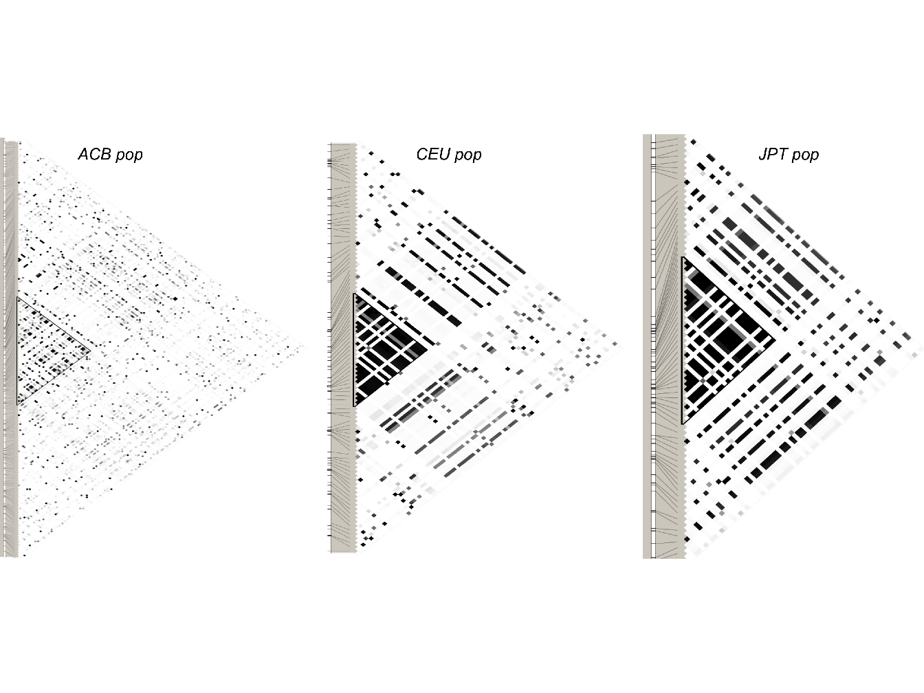
Figure 1.8: Plots of pairwise linkage disequilibrium for polymorphisms in the ACE (Angiotensin I Converting Enzyme) genomic region genotyped in three populations by the International HapMap Project. CEU, Utah residents with ancestry from northern and western Europe; ACB, African Caribbean in Barbados; JPT, Japanese in Tokyo; white, \(r^2\) = 0; black, \(r^2\) = 1; HapMap Release 22; chromosome 17 NCBI Build 37.

1.6.4 Origins of linkage disequilibrium

Founder mutations

Assume that a new mutation was introduced into the population at some point in the recent past. That mutation would have occurred on a single chromosome and would be transmitted with all alleles that are on the same chromosome, at least until recombination occurs. Thus, for many generations, the mutant allele would be associated with certain alleles at linked loci, and the strength of that association would diminish over time as a function of the recombination rate. If we look many generations later, the strength of the LD can be seen as an inverse measure of the distance between the loci. Of course, this presumes that the mutation was transmitted to an offspring and, through the process of genetic drift, expanded to sufficient prevalence to account for a significant burden of disease in present-day descendants of the affected founder.

Admixture

We consider a population that consists in a mixture of two subpopulations and two alleles, \(A\) and \(B\), having the following frequencies \(p_1 = q_1 = 0.9\) and \(p_2 = q_2 = 0.1\). If the two loci were independently distributed within each sub-population, then, in a 50-50 mixture of these two subpopulations, we would expect the following observed haplotypes distribution:

Through this example, we see an apparently very strong LD in the total population that is in fact spurious, leading to a complete artefact of population stratification. In statistical term, it is simply a reflection of Simpson’s paradox (Simpson 1951) or confounding by ethnicity in epidemiologic term.

Others factors that influence LD

Mutation and recombination may have the most evident impact on linkage disequilibrium, but there exist other factors that influence the distribution of disequilibrium. Most of these involve demographic aspects of a population, and tend to sever the relationship between LD strength and the physical distance between loci:

• Genetic drift: Increased drift of small, stable populations tends to increase LD, as haplotypes are lost from the population.

• Population growth: Rapid population growth decreases LD by reducing genetic drift.

• Gene flow: LD can be created by gene flow (migration) between populations. Initially, LD is proportional to the allele frequency differences between the populations, and is unrelated to the distance between markers. In the next generations, the “artificial” LD between unlinked markers quickly fades, while LD between nearby markers is more slowly broken down by recombination.

• Population structure: Various aspects of population structure are thought to influence LD. Population subdivision is likely to have been an important factor in establishing the patterns of LD in humans (Gabriel et al. 2002).

• Natural selection: There are two principal ways by which selection can affect the level of LD. The first is an hitchhiking effect (genetic draft) (Smith and Haigh 1974), in which an entire haplotype that flanks an advantageous variant can highly increase in frequency or even be fixed. Although the effect is generally weak, selection against deleterious variants can also inflate LD, as the deleterious haplotypes are swept from the population (Charlesworth, Morgan, and Charlesworth 1993). The second way in which selection can affect LD is through epistatic selection for combinations of alleles at two or more loci on the same chromosome. This form of selection leads to the association of particular alleles at different loci.

• Variable recombination rate: Recombination rates are known to vary by more than an order of magnitude across the genome. Because breakdown of LD is primarily driven by recombination, the extent of LD is expected to vary in inverse relation to the local recombination rate. It is even possible that recombination is largely confined to highly localized recombination hot spots, with little recombination elsewhere. According to this view, LD will be strong across the non-recombining regions and break down at hotspots.

References

Ardlie, K. G., L. Kruglyak, and M. Seielstad. 2002. “Patterns of Linkage Disequilibrium in the Human Genome.” Nature Reviews Genetics 3 (4): 299–309.

Barrett, Jeffrey C, B Fry, JDMJ Maller, and Mark J Daly. 2004. “Haploview: Analysis and Visualization of Ld and Haplotype Maps.” Bioinformatics 21 (2): 263–65.

Chapman, Juliet M, Jason D Cooper, John A Todd, and David G Clayton. 2003. “Detecting Disease Associations Due to Linkage Disequilibrium Using Haplotype Tags: A Class of Tests and the Determinants of Statistical Power.” Human Heredity 56 (1-3): 18–31.

Charlesworth, Brian, MT Morgan, and D Charlesworth. 1993. “The Effect of Deleterious Mutations on Neutral Molecular Variation.” Genetics 134 (4): 1289–1303.

Devlin, B, and Neil Risch. 1995. “A Comparison of Linkage Disequilibrium Measures for Fine-Scale Mapping.” Genomics 29 (2): 311–22.

Gabriel, S. B., S. F. Schaffner, H. Nguyen, J. M. Moore, J. Roy, B. Blumenstiel, J. Higgins, et al. 2002. “The Structure of Haplotype Blocks in the Human Genome.” Science 296 (5576): 2225–9.

Hedrick, Philip W. 1987. “Gametic Disequilibrium Measures: Proceed with Caution.” Genetics 117 (2): 331–41.

Hill, WG, and Alan Robertson. 1968. “Linkage Disequilibrium in Finite Populations.” Theoretical and Applied Genetics 38 (6): 226–31.

Hill, William G. 1974. “Estimation of Linkage Disequilibrium in Randomly Mating Populations.” Heredity 33 (2): 229.

Lewontin, R. C. 1964. “THE Interaction of Selection and Linkage. I. GENERAL Considerations; Heterotic Models.” Genetics 49 (1): 49–67.

Pritchard, Jonathan K, and Molly Przeworski. 2001. “Linkage Disequilibrium in Humans: Models and Data.” The American Journal of Human Genetics 69 (1): 1–14.

Robbins, RB. 1918. “Some Applications of Mathematics to Breeding Problems Iii.” Genetics 3 (4). http://europepmc.org/articles/PMC1200443.

Simpson, Edward H. 1951. “The Interpretation of Interaction in Contingency Tables.” Journal of the Royal Statistical Society. Series B (Methodological), 238–41.

Smith, John Maynard, and John Haigh. 1974. “The Hitch-Hiking Effect of a Favourable Gene.” Genetics Research 23 (1): 23–35.

Weir, Bruce S, and others. 1990. Genetic Data Analysis. Methods for Discrete Population Genetic Data. Sinauer Associates, Inc. Publishers.