1.5 Basic concepts in population genetics

1.5.1 Hardy-Weinberg equilibrium in large population

We consider a biallelic locus with alleles $A$ and $a$ present in a population at frequencies $p$ and $q$ respectively. If we assume that the two copies of the gene that an individual carries are inherited independently, then the number of copies of the allele $A$ will follow a binomial distribution, $\mathcal{B}(2,p)$, that is, that the probabilities of the three possible genotypes ($aa$, $aA$ and $AA$) will follow the Hardy-Weinberg law (Weinberg 1908):

\[p^2 + 2pq + q^2 = 1\]

with \[p^2 = p(AA); q^2 = p(aa) \mbox{ and } 2pq = p(Aa).\]

Hardy-Weinberg’s law states that in an isolated population of unlimited size, not subject to selection, and in which there are no mutations, the allelic frequencies remain constant. If the couplings are panmictic (random mating), the genotypic frequencies are deduced directly from the allelic frequencies and also remain constant. The assumption of random mating says that the probability that any pair of individual mates is unrelated to their genotype (except for the X chromosome) or their ethnic origin. However, in practice it is not truly the case since couples tend to mate within their ethnic group and are likely to select partners with compatible traits, some of which may be influenced by specific genes. Such non-random mating is commonly ignored in many genetic analyses of chronic disease traits, for which its effect may be negligible. Nevertheless, to the extent that it occurs, its major effect is to slow down the rate of convergence to Hardy-Weinberg equilibrium rather than to distort the equilibrium distribution (Thomas 2004).

Table 1.1: Expected frequency of an allele transmitted from an individual sampled from a population in Hardy-Weinberg Equilibrium
Parental Genotype	Genotype probability	Probability of transmitting A	Joint probability
AA	$p^2$	0	0
Aa	$2p(1-p)$	0.5	$p(1-p)$
aa	$(1-p)^2$	1	$(1-p)^2$
Total	1	-	p

1.5.2 Genetic drift in small population

In small populations, the results presented above will still be true in expectation, but the allele frequencies will vary from generation to generation simply as a result of chance (sampling error). It follows that, in finite populations, the expected value of the allele frequency will remain constant but its variance will increase from one generation to the next. This means that in generation, there is a non-zero probability that one allele might not be transmitted to any offspring, in which case that allele becomes extinct and the other becomes fixed. In fact, with absence of mutation and selection, one of the alleles will eventually become extinct, and the probability that it is the allele $a$ that disappears turns out to be simply $1 - q$.

At first glance, this might seem to contradict the claim that in expectation, the allele frequency remains constant, but in fact with probability $q$ the allele frequency will eventually become 1 and with probability $1 - q$ it will become 0; hence in expectation, the allele frequency remains $q \times 1 + (1 - q) \times 0 = q$. This phenomenon is known as genetic drift and was first introduced by Sewall Wright, one of the founders in the field of population genetics, (Wright 1929).

Figure 1.7 illustrates the effect of genetic drift on allelic frequencies for 2 alleles $A$ and $a$ at 1 locus for different population neither subject to selection nor mutation.

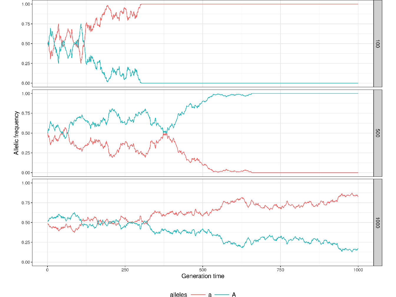
$Illustration of genetic drift in finite, small, populations. The plots show the evolution of allelic frequencies for 2 alleles $A$ and $a$ at 1 locus over 1000 generations for 3 population sizes (100, 500 and 1000). The 2 alleles are set to have the same proportions in the 3 populations at generation 1 ($p = q = 1/2$) and the frequencies of both allele evolve to be either fixed or extinct more or less quickly depending on the size of the population.$

Figure 1.7: Illustration of genetic drift in finite, small, populations. The plots show the evolution of allelic frequencies for 2 alleles $A$ and $a$ at 1 locus over 1000 generations for 3 population sizes (100, 500 and 1000). The 2 alleles are set to have the same proportions in the 3 populations at generation 1 ($p = q = 1/2$) and the frequencies of both allele evolve to be either fixed or extinct more or less quickly depending on the size of the population.

1.5.3 Concept of heritability

Sewall Wright and Ronald Fisher first introduced the concept of heritability in the context of family studies. Wright’s heritability is based on the analysis of correlation and its estimate is based on the path analysis method (Wright 1921) while the definition of Fisher is based on the analysis of variance and is defined as the proportion of total variance in a population for a particular measurement, taken at a particular time or age, that is attributable to variation in additive genetic or total genetic values (Fisher 1919).

An observed phenotype for a trait of interest can be partitioned into a statistical model representing the contribution of the unobserved genotype and unobserved environmental factors: \[\text{Phenotype} = \text{Genotype} + \text{Environment}.\]

The variance of the observed phenotype ($\sigma^2_P$) can thus be partitioned into the sum of unobserved genotype and environmental variances ($\sigma^2_G$ and $\sigma^2_E$): \[\sigma^2_P = \sigma^2_G + \sigma^2_E.\]

Following the definition of Fisher, the broad-sense heritability ($\text{H}^2$) can be expressed as a ratio of variances by expressing the proportion of the phenotypic variance that can be attributed to variance of genotypic values: \[\text{H}^2 = \frac{\sigma^2_G}{\sigma^2_P}.\]

The genetic variance $\sigma^2_G$ can further be partitioned into additive genetic effects ($\sigma^2_A$), dominance genetic effects ($\sigma^2_D$) and epistatic genetic effects ($\sigma^2_I$) and the narrow-sense heritability ($\text{h}^2$) is defined as: \[\text{h}^2 = \frac{\sigma^2_A}{\sigma^2_P}.\]

Heritabilities can be estimated from empirical data of the observed and expected resemblance between relatives. The expected resemblance between relatives depends on assumptions regarding its underlying environmental and genetic causes (Visscher, Hill, and Wray 2008). To estimate the heritability from population sample rather from family studies, we can resort on the use of the generalized linear mixed model (GLMM⁴), this heritability is known as the genomic heritability (Dandine-Roulland and Perdry 2015).

References

Dandine-Roulland, Claire, and Herve Perdry. 2015. “The Use of the Linear Mixed Model in Human Genetics.” Human Heredity 80 (4): 196–206.

Fisher, Ronald A. 1919. “XV.âThe Correlation Between Relatives on the Supposition of Mendelian Inheritance.” Earth and Environmental Science Transactions of the Royal Society of Edinburgh 52 (2): 399–433.

Mc Cullagh, Peter, and J. A. Nelder. 1989. “Generalized Linear Models, Second Edition.” CRC Press. https://www.crcpress.com/Generalized-Linear-Models-Second-Edition/McCullagh-Nelder/p/book/9780412317606.

Stroup, Walter W. 2012. Generalized Linear Mixed Models: Modern Concepts, Methods and Applications. CRC press.

Thomas, Duncan C. 2004. Statistical Methods in Genetic Epidemiology. Oxford University Press.

Visscher, Peter M., William G. Hill, and Naomi R. Wray. 2008. “Heritability in the Genomics Era-Concepts and Misconceptions.” Nature Reviews Genetics 9 (4): 255–66.

Weinberg, Wilhelm. 1908. “Ber Den Nachweis Der Vererbung Beim Menschen.” Jahres. Wiertt. Ver. Vaterl. Natkd. 64: 369–82.

Wright, Sewall. 1921. “Correlation and Causation.” Journal of Agricultural Research 20 (7): 557–85.

Wright, Sewall. 1929. “The Evolution of Dominance.” The American Naturalist 63 (689): 556–61.

The generalized linear mixed model is an extension of the generalized linear model (Mc Cullagh and Nelder 1989) in which the linear predictor contains random effects in addition to the usual fixed effects (see (Stroup 2012) for thorough introduction to GLMMs).↩