2.3 Parametric methods

2.3.1 Linear models

Linear models are statistical models where a univariate response $\mathbf{y} \in \mathbb{R}^n$ is modelled as the sum of $D$ linear predictor $\mathbf{X} \in \mathbb{R}^{n \times D}$ weighted by some unknown parameters, $\boldsymbol{\beta} \in \mathbb{R}^D$, which have to be estimated, and a zero mean random error term, $\boldsymbol{\epsilon}$. A linear model is generally written in the following matrix form:

\[\mathbf{y} = \boldsymbol{\beta}\mathrm{\mathbf{X}} + \boldsymbol{\epsilon}.\]

Statistical inference with such models is usually based on the assumption that the response variable has a normal distribution, i.e. \[\epsilon \sim \mathcal{N}(0, \mathbf{I}\sigma^2).\]

To estimate the unknown parameter, a sensible approach is to choose a value of $\boldsymbol{\beta}$ that makes the model fit closely the data. One possible way to proceed is to minimize a relevant cost function, defined by the residual sum of squares (RSS) of the model, with respect to $\boldsymbol{\beta}$, known as the least squares method (Gauss 1809): \[RSS(\boldsymbol{\beta}) = || \mathbf{y} - \mathbf{X} \boldsymbol{\beta}\ ||_2^2. \label{eq:RSS}\]

The least squares estimator is obtained by minimizing $RSS(\boldsymbol{\beta})$. To that end, we set the derivative of equal to zero to obtain the normal equations: \[\mathbf{X}^T\mathbf{X}\boldsymbol{\beta} = \mathbf{X}^T\mathbf{y}. \label{eq:normaleq}\]

Solving for $\boldsymbol{\beta}$, we obtain the ordinary least squares estimate: \[\hat{\boldsymbol{\beta}}^{OLS} = (\mathbf{X}^T\mathbf{X})^{-1}\mathbf{X}^T\mathbf{y},\] provided that the inverse of $\mathbf{X}^T\mathbf{X}$ exists, which means that the matrix $\mathbf{X}$ should have rank $D$. As $\mathbf{X}$ is an $n \times D$ matrix, this requires in particular that $n \geqslant D$, i.e. that the number of parameters is smaller than or equal to the number of observations.

2.3.2 Penalized linear regression

The Gauss-Markov theorem (Aitkin 1935) asserts that the least squares estimates $\hat{\boldsymbol{\beta}}^{OLS}$ have the smallest variance among all linear unbiased estimates. However, there may well exist biased estimators with smaller mean squared error that would trade a little bias for a larger reduction in variance. Subset selection, shrinkage methods (ridge regression, lasso regression, $\dots$) or dimension reduction approaches such as Principal Components Regression or Partial least Squares are useful approaches if we want to obtain such biased estimates with smaller variance. In this section we will only detailed the most commonly used shrinkage methods, as they are the ones used in association genetics.

Ridge regression

The least squares estimates are the best unbiased linear estimators but this estimation procedure is valid only if the correlation matrix $\mathbf{X}^T\mathbf{X}$ is close to a unit matrix or full-rank, i.e. when the predictors are not orthogonal. If not, (Hoerl and Kennard 1970) proposed to base the estimation of the regression parameters on the matrix $(\mathbf{X}^T\mathbf{X} + \lambda\mathbf{I})$, $\lambda \geq 0$ rather than on $\mathbf{X}^T\mathbf{X}$ and have developed the method named ridge regression to estimate the biased coefficients $\hat{\boldsymbol{\beta}}^{ridge}$. This method shrinks the coefficients of the regression towards zero by imposing a penalty on the sum of the squared coefficients. The ridge coefficients minimize a penalized residual sum of squares which can be written as follow:

\[\hat{\boldsymbol{\beta}}^{ridge} = \underset{\beta}{\text{argmin}} \left\lbrace || \mathbf{y} - \mathbf{X}\boldsymbol{\beta} ||_2^2 + \lambda ||\boldsymbol{\beta}||_2^2 \right\rbrace, \label{eq:ridge}\]

or can be equivalently written as a constrained problem: \[\underset{\beta}{\text{argmin}} \left\lbrace || \mathbf{y} - \mathbf{X}\boldsymbol{\beta} ||_2^2 \text{ subject to } \sum_{d=1}^D \boldsymbol{\beta}_d \leq t \right\rbrace,\] with $t \geqslant 0$ a size constraint and $\lambda \geqslant 0$ a penalty parameter that controls the amount of shrinkage: the larger the value of $\lambda$, the greater the amount of shrinkage. The ridge regression estimates can then be written as:

\[\boldsymbol{\hat{\boldsymbol{\beta}}}^{ridge} = (\mathbf{X}^T\mathbf{X} + \lambda \mathbf{I})^{-1} \mathbf{X}^T \mathbf{y}, \label{eq:ridgesol}\]

We can notice that the solution adds a positive constant to the diagonal of $\mathbf{X}^T\mathbf{X}$ before inversion, which makes the problem non-singular even if $\mathbf{X}^T\mathbf{X}$ is not full rank.

The penalty parameter $\lambda$ can be chosen either by $K$-fold cross-validation, leave-one-out cross-validation or by using the generalized cross-validation (Golub, Heath, and Wahba 1979). In generalized cross-validation, the estimate $\hat{\lambda}$ is the minimizer of $V(\lambda)$ given by \[V(\lambda) = \frac{1}{n} \frac{||(\mathbf{I} - \mathbf{A}(\lambda))\mathbf{y} ||_2^2}{\left[ 1/n \text{Trace}(\mathbf{I} - \mathbf{A}(\lambda))\right]^2},\] where $\mathbf{A}(\lambda) = \mathbf{X}(\mathbf{X}^T\mathbf{X} + n\lambda\mathbf{I})^{-1}\mathbf{X}^T$ and is known as the hat matrix.

Moreover (Hoerl and Kennard 1970) have shown that the total variance of the ridge coefficients decrease as $\lambda$ increases while the squared bias decrease with $\lambda$ and that there exists values $\lambda$ for which the MSE is less for $\hat{\boldsymbol{\beta}}^{ridge}$ than it is for $\hat{\boldsymbol{\beta}}^{OLS}$. These properties lead to the conclusion that it is advantageous to take a little bias to substantially reduce the variance and thereby improving the mean square error of estimation and prediction.

Lasso

The lasso (Tibshirani 1996) is also a shrinkage method but unlike ridge regression, it may set some coefficients to zero and thus perform variable selection. The lasso estimate is close to the ridge regression in the sense that it is a penalized linear regression with a penalty on the sum of the absolute value of the coefficients:

\[\hat{\boldsymbol{\beta}}^{lasso} = \underset{\boldsymbol{\beta}}{\text{argmin}} \left\lbrace || \mathbf{y} - \mathbf{X}\boldsymbol{\beta} ||_2^2 + \lambda ||\boldsymbol{\beta}||_1 \right\rbrace, \label{eq:lasso}\]

which can be equivalently written as the constrained problem: \[\underset{\boldsymbol{\beta}}{\text{argmin}} \left\lbrace || \mathbf{y} - \mathbf{X}\boldsymbol{\beta} ||_2^2 \text{ subject to } \sum_{d=1}^D |\beta_d| \leq t \right\rbrace,\] with $t \geqslant 0$ a size constraint and $\lambda \geqslant 0$ a penalty parameter.

Comparing and , we can see that the difference between lasso and ridge regression is found in the penalized term, the $||\boldsymbol{\beta}||_2^2$ term ($\ell_2$ squared norm) in ridge regression penalty has been replaced by $||\boldsymbol{\beta}||_1$ ($\ell_1$ norm) in the lasso penalty. The $\ell_1$ penalty has the effect of forcing some of the coefficient estimates to be exactly equal to 0 when the penalty parameter $\lambda$ is sufficiently large. This leads to sparse models much easily interpretable than those produced by ridge regression. Figure 2.2 illustrates how the lasso procedure can achieve sparsity while the ridge coefficients are only shrinking to zero.

However, the constraint put on the $\ell_1$ norm of the coefficients makes the solution of the lasso non-linear in $\mathbf{y}$ and therefore there is no closed form expression to calculate the solutions as in ridge regression. Efficient algorithms are available for computing the entire path of solutions as $\lambda$ varied, with the same computational cost as for the ridge regression (see homotopy methods (Osborne, Presnell, and Turlach 2000) such as LARS (Efron et al. 2004), or also proximal algorithms (Parikh, Boyd, and others 2014) for more details).

As for ridge regression, the tuning parameter $\lambda$ needs to be chosen but with the lasso we cannot rely on the generalized cross-validation to calculate the best value for $\lambda$. However, it is possible to use an ordinary cross-validation where we choose a grid of $\lambda$ values and compute the cross-validation error for each value of $\lambda$. We then select the tuning parameter for which the value of the cross-validation error is minimized and re-fit the model using all the available observations with the best $\lambda$.

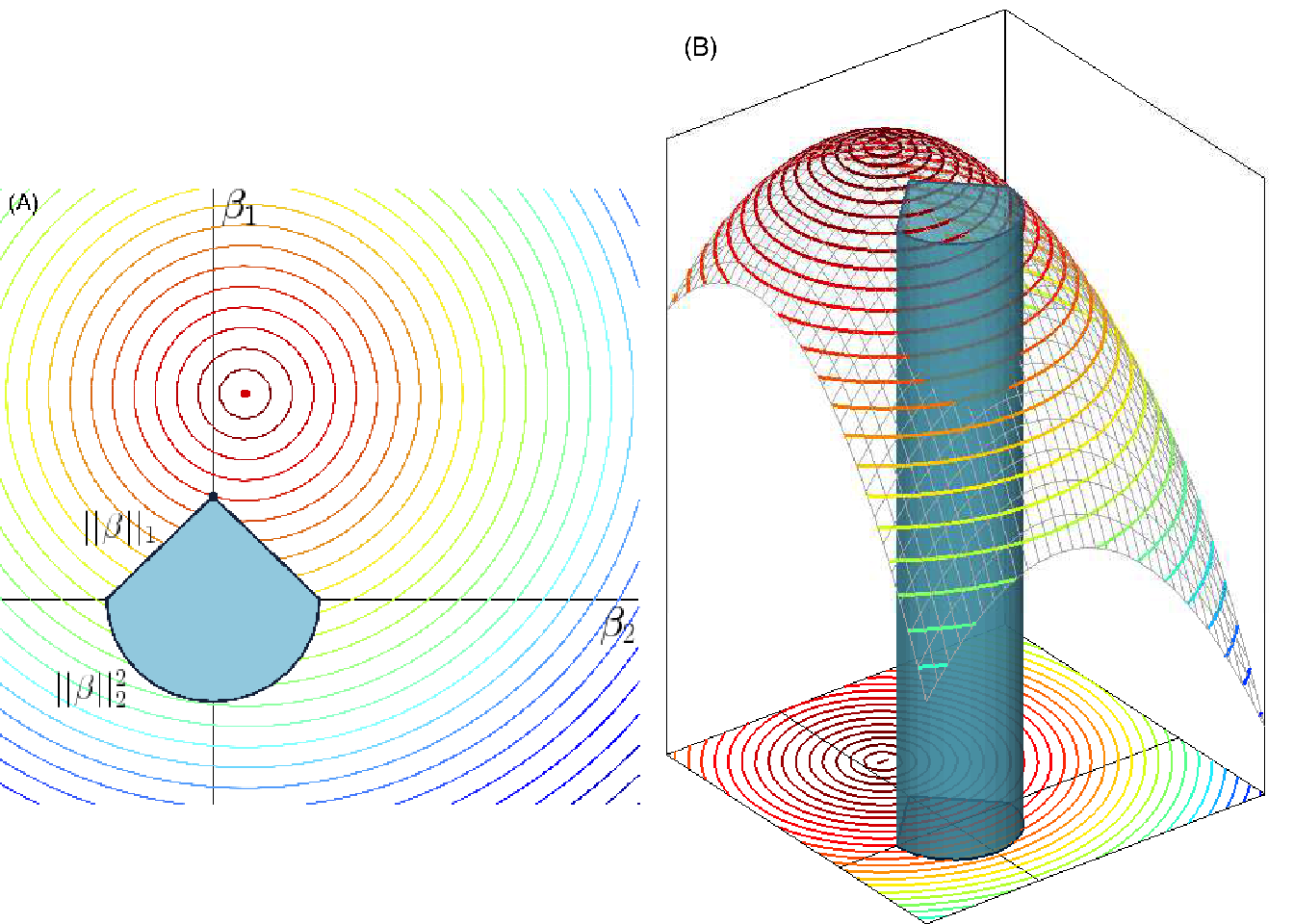
$Geometrical representation of sparsity in penalized linear regression. (A) A 2-dimensional representation of space of the coefficients $\beta_1$ and $\beta_2$. The blue geometric form represents two types of constraints, $||\beta||_1$ and $||\beta||^2_2$, applied to the coefficients. The circular coloured lines represent the contour of the cost function and the red dotted point is the true parameter $\beta$ we seek to reach. (B) 3-dimensional view of (A) where the constraints are represented as a tube in which the penalized methods are forced to stay to estimate the coefficients $\beta_1$ and $\beta_2$ (Image credit: Yves Grandvalet).$

Figure 2.2: Geometrical representation of sparsity in penalized linear regression. (A) A 2-dimensional representation of space of the coefficients $\beta_1$ and $\beta_2$. The blue geometric form represents two types of constraints, $||\beta||_1$ and $||\beta||^2_2$, applied to the coefficients. The circular coloured lines represent the contour of the cost function and the red dotted point is the true parameter $\beta$ we seek to reach. (B) 3-dimensional view of (A) where the constraints are represented as a tube in which the penalized methods are forced to stay to estimate the coefficients $\beta_1$ and $\beta_2$ (Image credit: Yves Grandvalet).

Group-Lasso

In some problems, the predictors belong to pre-identified groups; for instance genes that belong to the same biological pathway, SNP included in the same haplotype block or collections of indicator (dummy) variables for representing the levels of a categorical predictor. In this context it may be desirable to shrink and select the members of a group together. The group-lasso regression (Yuan and Lin 2006) is one way to achieve this.

If we suppose that $D$ predictors are divided into $G$ groups, with $p_g$ the number of variables in the group $g$ then the group-lasso solution minimizes the following penalized criterion:

\[\hat{\boldsymbol{\beta}}^{GL} = \underset{\boldsymbol{\beta}}{\text{argmin}} \left\lbrace || \mathbf{y} - \sum_{g=1}^G \mathbf{X}_g\boldsymbol{\beta}_g ||_2^2 + \lambda \sum_{g=1}^G \sqrt{p_g}||\beta_g||_2 \right\rbrace, \label{eq:group-lasso}\]

with $\mathbf{X}_g$ the matrix of predictors corresponding to the $g^{th}$ group, $\sqrt{p_g}$ the terms accounting for the varying groups sizes and $||\beta_g||_2$ the $\ell_2$-norm of the coefficients corresponding to group $g$. Since the Euclidean norm of a vector $\beta_g$ is zero only if all of its components are zero, this model encourages sparsity at the group level.

Generalizations include more general $\ell_2$ norms $||\nu^T||_K = (\nu^TK\nu)^{1/2}$ as well as overlapping groups of predictors (Jacob, Obozinski, and Vert 2009; Jenatton, Audibert, and Bach 2011).

2.3.3 Generalized linear models

Generalized linear models (GLMs) (Nelder and Wedderburn 1972) are an extension of linear models where the strict linearity assumption of linear models is somewhat relaxed by allowing the expected value of the response to depend on a smooth monotonic function of the linear predictor and has the basic structure: \[g(\theta) = \mathbf{X}\boldsymbol{\beta} = \beta_0 + \beta_1\boldsymbol{x}_1 + \dots + \beta_D\boldsymbol{x}_D,\] where $\theta \equiv \mathbb{E}(\mathrm{Y}|\mathrm{X})$, $g$ is a smooth monotonic ’link function’, $\mathbf{X}$ the $n \times D$ model matrix and $\boldsymbol{\beta}$ the unknown parameters. In addition, the assumption that the response should be normally distributed is also relaxed by allowing it to follow any distribution from the exponential family. The exponential family of distribution includes many distributions useful for practical modelling such as the Poisson, Binomial, Gamma and Normal distribution (see (Mc Cullagh and Nelder 1989) for comprehensive reference on GLMs). A distribution belongs to the exponential family of distributions if its probability density function can be written as \[g_{\theta}(\mathbf{y}) = \text{exp} \left[ \dfrac{\mathbf{y}\theta - b(\theta)}{a(\phi)} + c(\mathbf{y},\phi) \right],\] where $a$, $b$ and $c$ are arbitrary functions, $\phi$ the dispersion parameter and $\theta$ known as the canonical parameter of the distribution.

Furthermore, it can be shown that \[\mathbb{E}(\mathrm{Y}) = b'(\theta) = \mu, \label{eq:mu}\] and \[Var(\mathrm{y}) = b''(\theta)\phi. \label{eq:var}\]

Estimation and inference with GLMs are based on maximum likelihood estimation theory (RA Fisher 1922). The log-likelihood for the observed response $\mathbf{y}$ is given by \[l(f_{\theta}(\mathbf{y})) = \sum_{i=1}^n \dfrac{y_i\theta_i - b(\theta)}{a(\phi)} + c(y_i,\phi).\]

The maximum-likelihood estimate of $\boldsymbol{\beta}$ are obtained by partially differentiating $l$ with respect to each element of $\boldsymbol{\beta}$, setting the resulting expression to 0 and solving for $\boldsymbol{\beta}$: \[\dfrac{\partial l}{\partial \beta_d} = \sum_{i=1}^n \dfrac{(y_i - b'_i(\theta_i))}{\phi b''_i(\theta_i)} \dfrac{\partial \mu_i}{\partial \beta_d} = 0.\] Substituting and into this equation gives

\[\begin{equation} \sum_{i=1}^n \dfrac{(y_i - \mu_i)}{\text{Var}(\mu_i)} \dfrac{\partial \mu_i}{\partial \beta_d} = 0 \hspace{10pt} \forall d. \tag{2.1} \end{equation}\]

There are several iterative methods to solve the equation and estimate the maximum likelihood estimates $\hat{\beta_d}$. One can use the well-known Newton-Raphson method (Fletcher 1987), Fisher scoring method (Longford 1987) which is a form of Newton’s method or the Iteratively Reweighted Least Squares method developed by (Nelder and Wedderburn 1972).

Logistic regression

The logistic regression model (Cox 1958) is a generalized linear model where the logit function, defined as \[\text{logit}(t) = \log \left( \frac{t}{1-t} \right), \text{ with } t \in [0,1],\] is used as the ’link’ function for $g$ and is applied in the case where we want to model a qualitative random variable $\mathrm{Y}$ with $K$ classes. The logit function allows to model the posterior probability $\mathbb{P}(\mathrm{Y} = k)$ via linear function of the observations while at the same ensuring that they sum to one and remain in $[0,1]$. The model has the form:

\[\begin{aligned} \log \left( \frac{\mathbb{P}(\mathrm{Y} = 1 |\mathrm{X} = \boldsymbol{x})}{1 - \mathbb{P}(\mathrm{Y} = K |\mathrm{X} = \boldsymbol{x})} \right) & = \beta_{10} + \boldsymbol{\beta}_1^T \boldsymbol{x}, \\ \log \left( \frac{\mathbb{P}(\mathrm{Y} = 2 |\mathrm{X} = \boldsymbol{x})}{1 - \mathbb{P}(\mathrm{Y} = K |\mathrm{X} = \boldsymbol{x})} \right) & = \beta_{20} + \boldsymbol{\beta}_2^T\boldsymbol{x}, \\ \vdots \\ \log \left( \frac{\mathbb{P}(\mathrm{Y} = K-1 |\mathrm{X} = \boldsymbol{x})}{1 - \mathbb{P}(\mathrm{Y} = K |\mathrm{X} = \boldsymbol{x})} \right) & = \beta_{(K-1)0} + \boldsymbol{\beta}_{K-1}^T\boldsymbol{x} , \label{eq=logit}\end{aligned}\]

and equivalently \[\mathbb{P}(\mathrm{Y} = k |\mathrm{X} = \boldsymbol{x}) = \frac{\text{exp}(\beta_{k0} + \boldsymbol{\beta}_k^T\boldsymbol{x})}{1 + \sum_{k=1}^{K-1} \text{exp}(\beta_{k0} + \boldsymbol{\beta}_k^T\boldsymbol{x})}, \text{ with } k \in [1,\dots,K-1]. \label{eq=logit2}\]

When $K=2$ the model becomes simple since there is only a single linear function. It is widely used in biostatistics when we want to classify an individual as being a case or a control in genome-wide association studies for instance.

Logistic regression models are usually fit by maximum likelihood using the conditional likelihood of the response given the observations. In the two class case where $\mathbf{y}$ is encoded as $0/1$, the log-likelihood of the estimator can be written as:

\[\begin{aligned} l(\boldsymbol{\beta}) & = \sum_{i=1}^n \left[ y_i \log \left( \frac{e^{\boldsymbol{\beta}^T\boldsymbol{x}_i}}{1+e^{\boldsymbol{\beta}^T\boldsymbol{x}_i}}\right) + (1-y_i)\log \left( 1- \frac{e^{\boldsymbol{\beta}^T\boldsymbol{x}_i}}{1+e^{\boldsymbol{\beta}^T\boldsymbol{x}_i}} \right) \right] \\ & = \sum_{i=1}^n \left[ y_i\boldsymbol{\beta}^T\boldsymbol{x}_i - \log (1 + e^{\boldsymbol{\beta}^T\boldsymbol{x}_i}) \right]. \end{aligned}\]

References

Aitkin, AC. 1935. “On Least Squares and Linear Combination of Observations.” Proceedings of the Royal Society of Edinburgh 55: 42–48.

Cox, David R. 1958. “The Regression Analysis of Binary Sequences.” Journal of the Royal Statistical Society. Series B (Methodological), 215–42.

Efron, Bradley, Trevor Hastie, Iain Johnstone, Robert Tibshirani, and others. 2004. “Least Angle Regression.” The Annals of Statistics 32 (2): 407–99.

Fletcher, Roger. 1987. “Practical Methods of Optimization John Wiley & Sons.” New York 80.

Gauss, Carl Friedrich. 1809. Theoria Motus Corporum Coelestium in Sectionibus Conicis Solem Ambientium Auctore Carolo Friderico Gauss. sumtibus Frid. Perthes et IH Besser.

Golub, Gene H, Michael Heath, and Grace Wahba. 1979. “Generalized Cross-Validation as a Method for Choosing a Good Ridge Parameter.” Technometrics 21 (2): 215–23.

Hoerl, Arthur E, and Robert W Kennard. 1970. “Ridge Regression: Biased Estimation for Nonorthogonal Problems.” Technometrics 12 (1): 55–67.

Jacob, Laurent, Guillaume Obozinski, and Jean-Philippe Vert. 2009. “Group LAsso with Overlap and Graph LAsso.” In Proceedings of the 26th Annual International Conference on Machine Learning, 433–40. Montreal, Quebec, Canada.

Jenatton, Rodolphe, Jean-Yves Audibert, and Francis Bach. 2011. “Structured Variable Selection with Sparsity-Inducing Norms.” Journal of Machine Learning Research 12 (Oct): 2777–2824.

Longford, Nicholas T. 1987. “A Fast Scoring Algorithm for Maximum Likelihood Estimation in Unbalanced Mixed Models with Nested Random Effects.” Biometrika 74 (4): 817–27.

Mc Cullagh, Peter, and J. A. Nelder. 1989. “Generalized Linear Models, Second Edition.” CRC Press. https://www.crcpress.com/Generalized-Linear-Models-Second-Edition/McCullagh-Nelder/p/book/9780412317606.

Nelder, J. A., and R. W. M. Wedderburn. 1972. “Generalized Linear Models.” Journal of the Royal Statistical Society: Series A 135 (3): 370–84.

Osborne, Michael R, Brett Presnell, and Berwin A Turlach. 2000. “A New Approach to Variable Selection in Least Squares Problems.” IMA Journal of Numerical Analysis 20 (3): 389–403.

Parikh, Neal, Stephen Boyd, and others. 2014. “Proximal Algorithms.” Foundations and Trends in Optimization 1 (3): 127–239.

RA Fisher, MA. 1922. “On the Mathematical Foundations of Theoretical Statistics.” Phil. Trans. R. Soc. Lond. A 222 (594-604): 309–68.

Tibshirani, Robert. 1996. “Regression Shrinkage and Selection via the Lasso.” Journal of the Royal Statistical Society. Series B (Methodological) 58 (1): 267–88.

Yuan, Ming, and Yi Lin. 2006. “Model Selection and Estimation in Regression with Grouped Variables.” JOURNAL OF THE ROYAL STATISTICAL SOCIETY, SERIES B 68: 49–67.