2.2 Concepts of statistical learning
Assuming that there is some relationship between an observed response vector \(\mathbf{y} \in \mathbb{R}^n\) and \(D\) different predictors in \(\mathbf{X} \in \mathbb{R}^{n \times D}\), we can write this relationship in the very general from \[\mathbf{y} = f(\mathbf{X}) + \boldsymbol{\epsilon} ,\] where \(f\) : \(\mathcal{X} \rightarrow \mathcal{Y}\) is some fixed but unknown function of \(\mathbf{X}\) and \(\boldsymbol{\epsilon} \sim \mathcal{N}(0, \mathbf{I}\sigma^2)\) is a random error term, independent of \(\mathbf{X}\) and with \(\mathbf{I} \in \mathbb{R}^{n \times D}\) being the identity matrix.
By definition, statistical learning refers to a set of approaches designed to estimate \(f\) for 2 main reasons: prediction and explanation.
2.2.1 Prediction
In the setting where we have a set of input variables \(\mathbf{X}\) easily observable but where the output response \(\mathbf{y}\) cannot be readily obtained, then, since the error term averages to zero, \(\mathbf{y}\) can be predicted using \[\hat{\mathbf{y}} = \hat{f}(\mathbf{X}),\] where \(\hat{f}\) is the estimate of \(f\) and \(\hat{\mathbf{y}}\) is the resulting prediction for \(\mathbf{y}\). In this configuration, we are not especially concerned with the exact form of \(\hat{f}\) as long as it yields to an accurate prediction for \(\mathbf{y}\). In this context, we want to find a function \(\hat{f}\) that approximate the true function \(f\) as well as possible by means of statistical learning method. We will make “as well as possible” in the sense of minimizing a particular cost function which must reflect how accurate we are in predicting \(\mathbf{y}\). The most commonly used cost function in statistical regression is the mean-squared error (MSE) defined as: \[\| \mathbf{y} - \hat{f}(\mathbf{X})\|_2^2\]
Most of statistical learning methods aim to minimize the MSE (also known as the quadratic loss function) to estimate \(\hat{f}\) but other cost functions are also used in machine learning, depending on the task considered such as classification, regression or ranking (see for example the log loss, relative entropy, hinge loss, mean absolute error).
Bias-variance decomposition of mean squared error
Considering a couple of random variables \((\mathrm{X}, \mathrm{Y})\) defined on a training set \(\mathcal{T}\), then it can be shown that the expected mean squared error \(\mathbb{E}_\mathcal{T}[(\mathrm{Y} - \hat{f}(\mathrm{X}))^2]\), conditionally to \(\mathcal{T}\) and a noise term \(\epsilon\), can be parsed into two errors terms, bias and variance: \[\mathbb{E}_\mathcal{T}\lbrace[\mathrm{Y} - \hat{f}(\mathrm{X})]^2\rbrace = \underbrace{\mathbb{E}_\mathcal{T}[\hat{f}(\mathrm{X})^2] - \mathbb{E}^2_\mathcal{T}[\hat{f}(\mathrm{X})]}_{\text{Variance}(\hat{f}(\mathrm{X}))} + \underbrace{(\mathbb{E}_\mathcal{T}[\hat{f}(\mathrm{X})] - \mathbb{E}[f(\mathrm{X})])^2}_{\text{Bias}[\hat{f}(\mathrm{X})\rbrace} + \underbrace{\sigma^2}_{\text{Variance}(\epsilon)}.\]
Since the function \(\hat{f}\) has been constructed on a training set \(\mathcal{T}\), it is interesting to know how accurate it is on predicting \(\mathbf{y}\) when applied to a new data set, this measure is represented by the variance term in the MSE. Estimates with high variance will tend to perform poorly when seeing new data, in general more complex models tend to have a higher variance.
On the other hand, the bias error term refers to the error that is introduced by approximating the real, generally complex, function \(f\). For instance, if we try to approximate a non-linear function using a learning method designed for linear models, there will be error in the estimate \(\hat{f}\) due to this assumption. The more complex the model is, the lower the bias will be but at a cost of a higher variance.
That is why when we try to fit a model on some data, we always search for the best compromise between variance and bias (the so-called bias-variance trade-off) and therefore between complexity and simplicity. The fact that highly complex models have a lower bias but generalize poorly on new data is known as overfitting and occurs when the model fit too closely the data, going so far as to interpolate them in the most extreme case (see Figure 2.1 for an illustration of bias-variance trade-off).
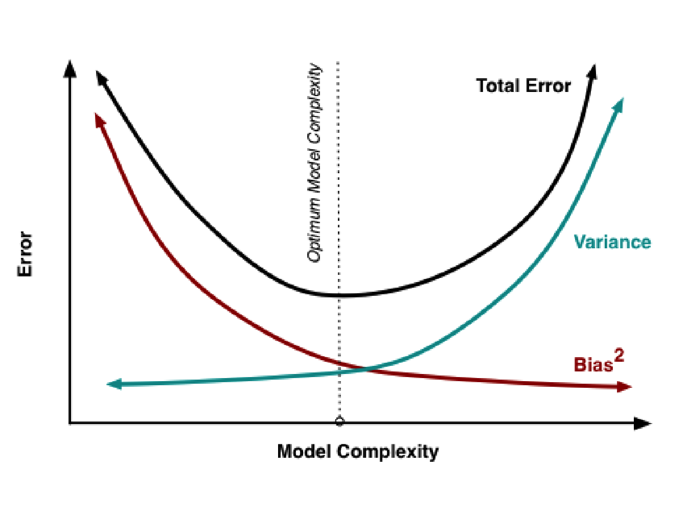
Figure 2.1: Bias and variance contribution to the total error. The bias (red curve) decreases as the model complexity increases unlike variance, which increases. The vertical dotted line shows the optimal model complexity, i.e. where the error criterion is minimized (image taken from http://scott.fortmann-roe.com/docs/BiasVariance.html).
The last term, \(\sigma^2\), corresponds to the variance of the noise, also called the irreducible error because the response variable is also a function of \(\epsilon\) which, by definition, cannot be predicted using the observations. Since all terms are non-negative, this error forms a lower bound on the expected error on unseen samples (Friedman, Hastie, and Tibshirani 2001).
Explanation
We can also be interested in understanding the relationship between \(\mathrm{Y}\) and \(\mathrm{X}\). In this situation we are more interested by the exact form of \(\hat{f}\) and we may want to answer the following questions: Which predictors are associated with the response? What is the relationship between the response and each predictor? Can the relationship be described using a linear equation or with a non-linear smoother? To answer these questions, we will tend to use more interpretable, i.e. simpler, models and to rely on the theory of hypothesis testing developed by (Neyman and Pearson 1933). We will introduce the theory of hypothesis testing and the most common tests in Section 2.6.
Estimation of \(f\)
All statistical learning methods can be roughly characterized as either parametric or non-parametric.
Parametric methods: They are model-based approaches that reduce the problem of estimating \(f\) down to estimating a set of parameters. Assuming a parametric form for \(f\) simplifies the estimation problem because it is generally easier to estimate a set of parameters, as in the linear model, than to fit an entirely arbitrary function. The main drawback is that the chosen model is generally too far for the true form of \(f\) leading to a poor estimate. Even if more flexible models, such as polynomial models, can fit more closely the true form of \(f\), they require in general to estimate a greater number of parameters which can lead to overfit the data, meaning that they follow the errors to closely and cannot be generalized to other data. We will present in Section 2.3.1 the linear model with its extension known as generalized linear models and some penalized approaches in Section 2.3.2.
Non-parametric methods: These approaches do not make explicit assumptions about the functional form of \(f\) but instead seek an estimate that fit closely the data to some degree to avoid overfitting. These methods have the advantage of being able to fit a wider range of form for \(f\) since no assumption about the functional form for \(f\) is made. However, they require a larger number of observations than is typically needed for a parametric approach to obtain an accurate estimate for \(f\). We will present in Section 2.4 some non-parametric models such as the regression splines and the generalized additive model5.
References
Friedman, Jerome, Trevor Hastie, and Robert Tibshirani. 2001. The Elements of Statistical Learning. Vol. 1. Springer series in statistics New York.
Neyman, Jerzy, and Egon S Pearson. 1933. “The Testing of Statistical Hypotheses in Relation to Probabilities a Priori.” In Mathematical Proceedings of the Cambridge Philosophical Society, 29:492–510. Cambridge University Press.
To be more specific, we will present the semi-parametric forms of these models using a linear basis expansion.↩