5.3 Method
In this section, we provide some elements to enhance Problem for biological problems involving metagenomic and genomic data. After a brief discussion related to the preprocessing of the data, we explain how to obtain the group structure on \(\mathit{G}\) and \(\mathit{M}\) using hierarchical clustering strategies and describe how to efficiently take into account the different scales of the groups defined by each level of the hierarchies. We then present some compressions that may be used to summarize the groups. Finally, we propose a linear model testing to recover the relevant interactions.
We entitled the proposed approach SICOMORE for Selection of Interaction
effects in COmpressed Multiple Omics REpresentations, implemented in the
R package SICoMORe available at https://github.com/fguinot/sicomore-pkg.
5.3.1 Preprocessing of the data
To tackle problems that involve genomic and metagenomic interactions, some prior transformations are mandatory. Also, a first attempt to reduce the dimension may be achieved at this step.
5.3.2 Preprocessing of metagenomic data
5.3.2.1 Normalization.
In shotgun metagenomics,17 microorganisms are studied by sequencing DNA fragments directly from samples, without the need for cultivation of individual isolates (Sharpton 2014).
Shotgun metagenomic sequencing data are often produced by analysing the presence of genes and their abundances in and between samples from different experimental conditions. The gene abundances are then estimated by matching each generated sequence read against a comprehensive and annotated reference database and by counting the number of reads matching each gene in the reference database (Pereira et al. 2018).
Gene abundance data generated by such analysis are however affected by systematic variability that significantly increases the variation between samples and thereby decrease the ability to identify genes that differ in abundance (Jonsson et al. 2017; Wooley, Godzik, and Friedberg 2010; Pereira et al. 2018). The process known as normalisation therefore referred to the methods designed to remove such systematic variability.
A wide range of different methods has been applied to normalize shotgun metagenomic data. The majority of these normalization methods are based on scaling, where a sample-specific factor is estimated and then used to correct the gene abundances. For instance, one can simply calculates the scaling factor \(\psi_i\) as the sum of all reads counts in a sample \(i\): \[\psi_i = \sum_{j=1}^{D_{\mathit{M}}} x_{ij}^{\mathit{M}}.\]
A more robust method to estimate the scaling factor is the Trimmed Mean of M-values (TMM) (Robinson and Oshlack 2010) which compares the gene abundances in the samples against a reference, typically set as one of the samples in the study. We note \(t_i\) the scaling normalization factors for raw library sizes calculated using the TMM normalization method for sample \(i\); \(l_i = \mathbf{x}_i^{\mathit{M}} t_i\) is then the corresponding normalized library size for sample \(i\) and \[\psi_i = \frac{l_i}{\sum_{t=1}^n l_t/n},\] is the associated normalization scaling factor.
The raw counts \(x_{ij}^{\mathit{M}}\), with \(j \in [1, \dots, D_{\mathit{M}}]\), are then divided by the scaling factor to obtain the normalized counts: \[\tilde{x}_{ij}^{\mathit{M}} = x_{ij}^{\mathit{M}}/\psi_i .\]
5.3.2.2 Transformation.
Metagenomic shotgun sequencing results in features which take the form of proportions in different samples, referred in the statistical literature as compositional data (Aitchison 1982). These data are known to be subject to negative correlation bias (Pearson 1896; Aitchison 1982)) and the assumption of conditional independence among samples is unlikely to be true for the vast majority of metagenomic datasets.
Several data transformations have been suggested for RNA-seq data, most often in the context of exploratory or differential analyses. These transformations include log transformation (where a small constant is typically added to read counts to avoid 0’s), a variance-stabilizing transformation (Tibshirani 1988; Huber et al. 2003), moderated log counts per million (Law et al. 2014), and a regularized log-transformation (Love, Huber, and Anders 2014).
(Rau and Maugis-Rabusseau 2017) also proposed to calculate normalized expression profiles for each feature, that is, the proportion of normalized reads observed for gene \(j\) with respect to the sum of all samples in gene \(j\):
\[p_{ij} = \frac{\tilde{x}_{ij}^{\mathit{M}} + 1}{\sum_{t=1}^n \tilde{x}_{tj}^{\mathit{M}} + 1},\] where a constant of 1 is added to the numerator and denominator due to the presence of 0 counts.
However, the vector of values \(\mathbf{p}_j\) are linearly dependent, which imposes constraints on the covariance matrices that can be problematic for most standard statistical approaches (Rau and Maugis-Rabusseau 2017). One solution is to apply the commonly used centered log ratio (CLR) transformation for compositional data (Aitchison 1982). It is defined as: \[\text{CLR}(\mathbf{p}_j) = \left[ \ln\left( \frac{p_{1j}}{g(\mathbf{p}_j)}\right) , \dots, \ln\left( \frac{p_{nj}}{g(\mathbf{p}_j)}\right) \right],\] where \(g(\mathbf{p}_j)\) is the geometric mean of \(\mathbf{p}_j\).
5.3.2.3 A first selection of variables
As seen in Section 5.2, we assume strong dependencies on interactions, which means that an interaction can be effective only if the two simple effects making up the interaction are involved in the problem. Then, it may be clever to apply a first process of selection to discard the inoperative single effects on \(\mathit{G}\) and \(\mathit{M}\) respectively. Different approaches may be envisioned to proceed this selection. Among them, screening rules can eliminate variables that will not contribute to the optimal solution of a sparse problem sweeping all the variables upstream to the optimization. When such a screening is appropriate, we may use the work of (Lee et al. 2017) focused on Lasso problems, which present a recent overview of these techniques together with a screening rule ensemble. Once the screening is done, the optimization of a Lasso problem gives the final set of variables.
5.3.3 Structuring the data
Once the data are preprocessed, we can resort to hierarchical clustering using Ward criterion with appropriate distances to uncover the tree structures.
5.3.3.1 Clustering of metagenomic data
A common approach to analyse metagenomic data is to group sequences into taxonomic units. The features stemming from metagenome sequencing are often modelled as Operational Taxonomic Units (OTU), each OTU representing a biological species according to some degree of taxonomic similarity. (Chen et al. 2013) propose a comparison of methods to identify OTU that includes hierarchical clustering. While the structure on microbial species could be defined according to the underlying phylogenetic tree, it also makes sense to use more classical distances, such as the Ward criterion, to define a hierarchy based on the abundances of OTU. In our application we use an agglomerative hierarchical clustering with the Ward criterion (see Section 2.5.1).
5.3.3.2 Clustering of genomic markers
On the other hand, when the genomic information is available through SNP, the tree structure on \(\mathit{G}\) will be defined using a Ward spatially constrained hierarchical clustering algorithm which integrates the linkage disequilibrium as the measure of dissimilarity using the adjclust algorithm (A. Dehman, Ambroise, and Neuvial 2015).
5.3.4 Using the structure efficiently
Different approaches related to the problem of finding an optimal number of clusters may be envisioned to find the optimal cut in a tree structure obtained with hierarchical clustering (see for instance (Milligan and Cooper 1985) or (Gordon 1999)). Whatever the chosen approach, a systematic exploration of different levels of the hierarchy is mandatory to find this optimal cut. We define an alternative strategy to bypass this expensive exploration which consists in:
- Expanding the hierarchy considering all possible groups at a single level;
- Assigning a weight to each group based on gap distances between two consecutive groups in the hierarchy;
- Compressing each group into a supervariable.
The different steps of this strategy are illustrated in Figure 5.1, from the original tree structure in Figure 5.1(a) to a final flatten, weighted and compressed representation in Figure 5.1(c).
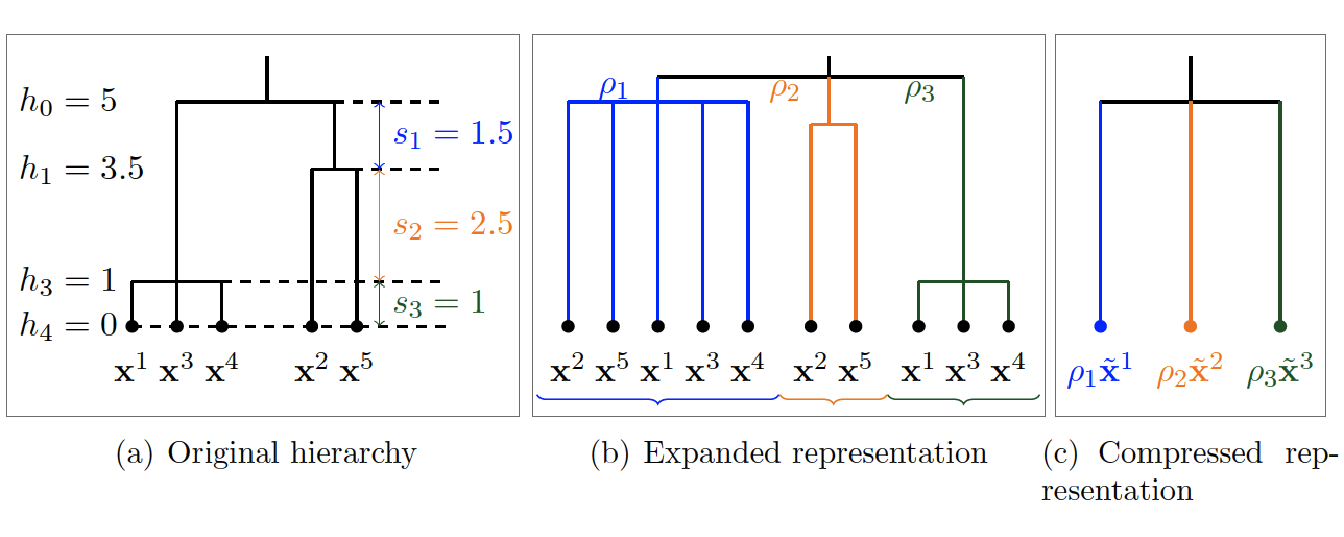
Figure 5.1: Dimension reduction strategy. (a) Original hierarchical tree with an example for 5 variables. (b) Expanded representation of the tree with all possible weighted groups derived from the original hierarchy. (c) Compressed representation of the tree after construction of the supervariables.
Expanding the hierarchy
To reduce the dimension involved in Problem , the first step consists in flattening the respective tree structures obtained on views \(\mathit{G}\) and \(\mathit{M}\) so that only a group structure remains. Thus, each group of variables defined at the deepest level may be included in other groups of larger scales, as shown in Figure 5.1(b).
Assigning weights to the groups
To keep track of the tree structure, we may integrate an additional measure quantifying the quality of the groups on two successive levels. More specifically, for a tree structure of height \(H\) and for \(1 \leq h \leq H-1\), we define \(s_h\) as the gap between heights \(s_h\) and \(s_{h-1}\). Following the lines of (Grimonprez 2016) for the Multi-Layer Group-Lasso described in Section 2.5.3, we define this quantity as \(\displaystyle{\rho_h = 1 / \sqrt{s_h}}\). The process is shown in Figure 5.1(a) and 5.1(c).
Compressing the data
To summarize each group of variables, the mean, the median or other quantiles may be used as well as more sophisticated representations based on eigen values decompositions such as the first factor obtained with a PCA. This step is similar to the dimension reduction step of the method presented in Section 4.2.2.
5.3.5 Identification of relevant supervariables
With this compressed representation at hand, we can recover relevant interactions with a multiple testing strategy.
Selection of supervariables
The compression is a key ingredient to reduce significantly the dimension involved in Problem . Yet, we are going a step further with an additional feature selection process applied to the compressed variables, as suggested at the begin of this section to preprocess the data, using screening rules and / or applying a Lasso optimization on each view \(\mathit{G}\) and \(\mathit{M}\): \[\begin{aligned} \underset{\boldsymbol{\beta}_{\mathit{G}}}{argmin} & \; \sum_{i=1}^n \left(y_i - \tilde{\mathbf{x}}_{i}^{\mathit{G}} \boldsymbol{\beta}_{\mathit{G}} \right)^2 \ + \ \lambda_{\mathit{G}} \sum_{g=1}^{N_{\mathit{G}}} \rho_g |\beta_{g}| \,,\end{aligned}\] and \[\begin{aligned} \underset{\boldsymbol{\beta}_{\mathit{M}}}{argmin} & \; \sum_{i=1}^n \left(y_i - \tilde{\mathbf{x}}_{i}^{\mathit{M}} \boldsymbol{\beta}_{\mathit{M}} \right)^2 \ + \ \lambda_{\mathit{M}}\sum_{m=1}^{N_{\mathit{M}}} \rho_m |\beta_{m}| \,, \end{aligned}\] with penalty factors being defined by \(\displaystyle{\rho_g = 1 / \sqrt{s_g}}\) and \(\displaystyle{\rho_m = 1 / \sqrt{s_m}}\) as explained in Section 5.3.3.
Linear model testing
In a feature selection perspective, the relevant interactions may be recovered separately considering each selected group \(g \in \mathcal{G}\) coupled with each selected group \(m \in \mathcal{M}\) in a linear model of interaction and by performing an hypothesis test on the interaction parameter: \[\label{eq:compact_single_interaction_model} y_i = \tilde{x}_i^g \beta_{g} + \tilde{x}_i^m \beta_{m} + \left(\tilde{x}_i^g \cdot \tilde{x}_i^m\right) {\theta_{gm}} + \, \epsilon_i \,.\]
This strategy has the advantage of highlighting all the potential interactions between the selected simple effects in an exploratory rather than predictive analysis perspective. Also, it may be regarded as an alternative shortcut to Problem in that it involves \(N_I\) problems of dimension \(3\) instead of a potentially large problem of dimension \(N_{\mathit{G}} + N_{\mathit{M}} + N_I\). Finally, this scheme of selection preserves strong dependencies by construction.
References
Aitchison, Jonh. 1982. “The Statistical Analysis of Compositional Data.” Journal of the Royal Statistical Society. Series B (Methodological) 44 (2): 139–77.
Chen, Wei, Clarence K. Zhang, Yongmei Cheng, Shaowu Zhang, and Hongyu Zhao. 2013. “A Comparison of Methods for Clustering 16S rRNA Sequences into OTUs.” PLoS ONE 8 (8): e70837.
Dehman, A., C. Ambroise, and P. Neuvial. 2015. “Performance of a Blockwise Approach in Variable Selection Using Linkage Disequilibrium Information.” BMC Bioinformatics 16: 148.
Gordon, Aharon D. 1999. Classification. Monographs on Statistics and Applied Probability. Chapman & Hall.
Grimonprez, Quentin. 2016. “Selection de Groupes de Variables corrélées En Grande Dimension.” PhD thesis, Université de Lille; Lille 1.
Huber, Wolfgang, Anja von Heydebreck, Holger Sültmann, Annemarie Poustka, and Martin Vingron. 2003. “Parameter Estimation for the Calibration and Variance Stabilization of Microarray Data.” Statistical Applications in Genetics and Molecular Biology 2 (1).
Jonsson, Viktor, Tobias Österlund, Olle Nerman, and Erik Kristiansson. 2017. “Variability in Metagenomic Count Data and Its Influence on the Identification of Differentially Abundant Genes.” Journal of Computational Biology 24 (4): 311–26.
Law, Charity W, Yunshun Chen, Wei Shi, and Gordon K Smyth. 2014. “Voom: Precision Weights Unlock Linear Model Analysis Tools for Rna-Seq Read Counts.” Genome Biology 15 (2): R29.
Lee, Seunghak, Nico Görnitz, Eric P. Xing, David Heckerman, and Christoph Lippert. 2017. “Ensembles of LAsso Screening Rules.” IEEE Transactions on Pattern Analysis and Machine Intelligence PP (99): 1–1.
Love, Michael I, Wolfgang Huber, and Simon Anders. 2014. “Moderated Estimation of Fold Change and Dispersion for Rna-Seq Data with Deseq2.” Genome Biology 15 (12): 550.
Milligan, Glenn W., and Martha C. Cooper. 1985. “An Examination of Procedures for Determining the Number of Clusters in a Data Set.” Psychometrika 50 (2): 159–79.
Pearson, Karl. 1896. “Mathematical Contributions to the Theory of Evolution. On a Form of Spurious Correlation Which May Arise When Indices Are Used in the Measurement of Organs.” Proceedings of the Royal Society of London 60: 489–98.
Pereira, Mariana Buongermino, Mikael Wallroth, Viktor Jonsson, and Erik Kristiansson. 2018. “Comparison of Normalization Methods for the Analysis of Metagenomic Gene Abundance Data.” BMC Genomics 19 (1): 274.
Rau, Andrea, and Cathy Maugis-Rabusseau. 2017. “Transformation and Model Choice for Rna-Seq Co-Expression Analysis.” Briefings in Bioinformatics 19 (3): 425–36.
Robinson, Mark D, and Alicia Oshlack. 2010. “A Scaling Normalization Method for Differential Expression Analysis of Rna-Seq Data.” Genome Biology 11 (3): R25.
Sharpton, Thomas J. 2014. “An Introduction to the Analysis of Shotgun Metagenomic Data.” Frontiers in Plant Science 5: 209.
Tibshirani, Robert. 1988. “Estimating Transformations for Regression via Additivity and Variance Stabilization.” Journal of the American Statistical Association 83 (402): 394–405.
Wooley, John C, Adam Godzik, and Iddo Friedberg. 2010. “A Primer on Metagenomics.” PLoS Computational Biology 6 (2): e1000667.