2.4 Splines and generalized additive models: Moving beyond linearit

2.4.1 Introduction

So far, we have been interested in estimating a function \(\hat{f}\) linear in \(\mathbf{X}\), but in reality, it is unlikely to be true. Linear models have the advantage of being easily interpretable and the approximation of \(f\) by a simple linear function can avoid overfitting. On the other hand, when the true function is highly non-linear, they are often limited if one wants to be able to model a complex phenomenon or to make accurate prediction.

In this section we will describe some methods that allow to take into account the non-linear form of \(f\) by working on a linear basis expansion of the initial features. The idea is to augment/replace the matrix of inputs \(\mathbf{X}\) with additional variables, which are transformations of \(\mathbf{X}\), and then use linear models in this new space of derived input variables.

We define the linear basis expansion of \(x \in \mathbb{R}\) by: \[s(x) = \sum_{k=1}^K \beta_k h_k(x),\] with \(h_k(x) : \mathbb{R} \mapsto \mathbb{R}\) the \(k^{th}\) transformation of \(x\), \(k \in [1, \dots, K]\). The function \(s(\mathbf{x})\) is also referred as a smoother since it produces an estimate of the trend that is less variables than the response variable \(\mathbf{y}\) itself. We call the estimate produced by a smoother a smooth.

The linear basis expansion offers a wide range of possible transformations for \(x\) such as:

• Third order polynomial transformation: \(h_1(x) = x, h_2(x) = x^2, h_3(x) = x^3\),

• non-linear transformation: \(h_k(x) = \text{log}(x), \sqrt{x}, \dots\),

• Piecewise constant transformation: \(h_1(x) = I(x < \xi_1), h_2(x) = I(\xi_1 \leq x \leq \xi_2), \dots, h_K(x) = I(x \geq \xi_{K-1})\).

In the following sections we will present some methods based on the linear basis expansion such as the regression splines (Section 2.4.2, smoothing splines (Section 2.4.4 and generalized additive models (Section 2.4.5). Note that the splines are methods applied to a univariate function \(x\) while the generalized additive models extend the uses of splines and other non-linear functions to the multivariate case.

2.4.2 Regression splines

Piecewise polynomials regression splines

Here the data are divided into different regions, each being defined by a polynomial function and separated by a sequence of knots, \(\xi_1, \xi_2, \dots, \xi_K\) and each piece are smoothly joined at those knots. For example, with one knot \(\xi\), dividing the data into two regions and with third-order polynomial pieces, we can write:

\[ s(x) = \left\{ \begin{array}{ll} \beta_{01} + \beta_{11}x + \beta_{21}x^2 + \beta_{31}x^3 + \epsilon \text{ if } x < \xi, \\ \beta_{02} + \beta_{12}x + \beta_{22}x^2 + \beta_{32}x^3 + \epsilon \text{ if } x > \xi. \\ \end{array} \right. \]

Piecewise cubic polynomials are generally used and constrained to be continuous and to have continuous first and second derivatives at the knots. For any given set of knots, the smooth is computed by multiple regression on an appropriate set of basis vectors. These vectors are the basis functions representing the family of piecewise cubic polynomials, evaluated at the observed values of the predictor \(x\).

Cubic regression splines

A simple choice of basis functions for piecewise-cubic splines (truncated power series basis) derives from the parametric expression for the smooth

\[s(\boldsymbol{x}) = \beta_0 + \beta_1x + \beta_2x^2 + \beta_3x^3 + \sum_{k=1}^{\mathit{K}}\beta_k(x - \xi_k)_+^3, \label{eq:cubic}\]

which have the required properties:

• \(s\) is cubic polynomial in any subinterval \([\xi_k,\xi_{k+1}]\),

• \(s\) has two continuous derivatives,

• \(s\) has a third derivative that is a step function with jumps at \(\xi_1,\dots,\xi_{\mathit{K}}\).

The sequence of knots can be placed over the range of the data or at appropriate quantiles of the predictor variable (e.g., 3 interior knots at the three quartiles).

A cubic spline satisfies the following properties:

\[s(x) \in C^2[\xi_0,\xi_n] = \left\{ \begin{array}{ll} s_{0}(x), \hspace{.5cm} \xi_0 \leq x \leq \xi_1, \\ s_{1}(x), \hspace{.5cm} \xi_1 \leq x \leq \xi_2, \\ \dots\\ s_{n-1}(x), \hspace{.5cm} \xi_{n-1} \leq x \leq \xi_n, \\ \end{array} \right.\] and

\[s(x): \left\{ \begin{array}{ll} s_{k-1}(x_k) = s_k(x_k) \\ s'_{k-1}(x_k) = s'_k(x_k) \\ s''_{k-1}(x_k) = s''_k(x_k) \\ \end{array} \right. ,\text{ for } k = 1,2,\dots,(n-1).\]

The choice of a third-order polynomial allows the function \(s(x)\) to be continuous at the knots.

Natural splines

A variant of polynomial splines are the natural splines: these are simply splines with an additional constraint that forces the function to be linear beyond the boundary knots. It is common to supply an additional knot at each extreme of the data and impose linearity beyond them. Then, with \(K-2\) interior knots (and two boundary knots), the dimension of the space of fits is \(K\). The lesser flexibility at the boundaries of natural splines tends to decrease the variance we can get when fitting regular regression splines.

We add the following condition to get a natural cubic spline: \[s''(\xi_0) = s''(\xi_n) = 0.\]

Figure 2.3 illustrates the use of natural cubic splines for the construction of an interpolating smooth curve.

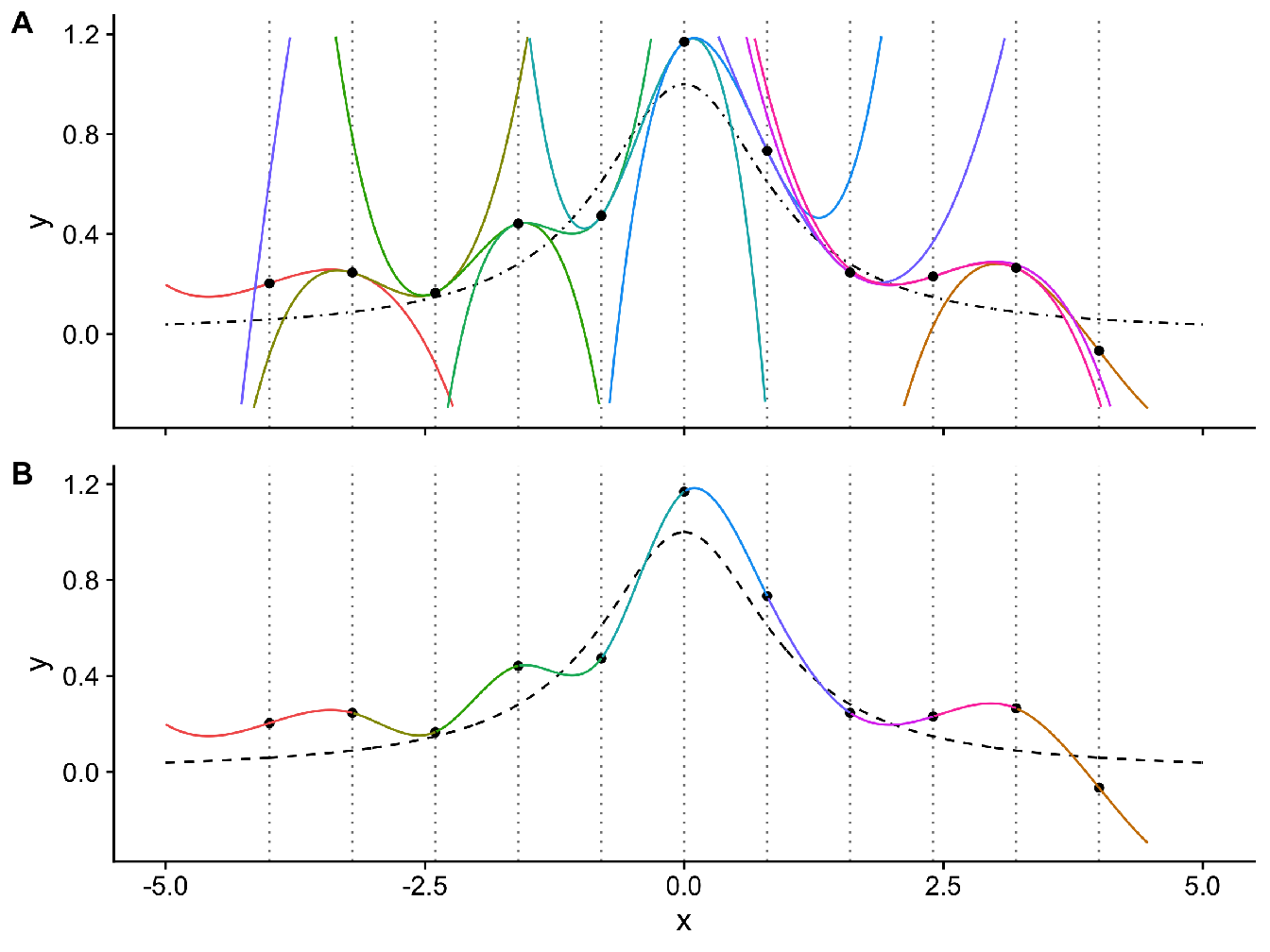
Figure 2.3: The black dashed line corresponds to the true distribution \(y = \frac{1}{1+x^2}\) and each \(n = 11\) black dots correspond to observations drawn from this distribution (with a little noise). In (A) we have represented the polynomial functions at each \(K = 11\) knots, constituting the natural cubic splines basis and (B) the truncated polynomials to construct the smoother.

2.4.3 \(\mathrm{B}\)-splines

The \(\mathrm{B}\)-spline basis functions provide a numerically superior alternative basis to the truncated power series. Their main feature is that any given basis function \(\mathit{B}_k(x)\) is non-zero over a span of at most five distinct knots which means that the resulting basis function matrix \(\mathbf{B}\) is banded. The \(\mathit{B}_k\) are piecewise cubics and we need \(K + 4\) of them (\(K + 2\) for natural splines) if we want to span the entire space. The algebraic definition is detailed in (Boor 1975).

With the \(\mathrm{B}\)-spline basis, the functions are strictly local - each basis is only non-zero over the interval between \(m+3\) adjacent knots, where \(m\) is the order of the basis (\(m = 2\) for cubic spline). To define a \(K\) parameters \(\mathrm{B}\)-spline basis, we need to define \(k+m+1\) knots, \(x_1 < x_2 < \dots < x_{m+k+1}\), where the interval over which the spline is to be evaluated lies within \([x_{m+2},x_k]\) (so that the first and last \(m+1\) knot locations are essentially arbitrary). An \((m+1)^{th}\) order \(\mathrm{B}\)-spline can be represented as

\[s(x) = \sum_{k=1}^K B_k^m(x)\beta_k,\] where the \(\mathrm{B}\)-spline basis functions are most conveniently defined recursively as follows:

\[B_k^m (x) = \frac{x-x_k}{x_{k+m+1} - x_k}B_k^{k-1}(x) + \frac{x_{k+m+2} - x}{x_{k+m+2}-x_{k+1}}B_{k+1}^{x-1}(\boldsymbol{x}) \hspace{.5cm} \text{for } k=1,\dots,K,\] and

\[B_k^{-1}(x) = \left\{ \begin{array}{ll} 1 \hspace{1cm} x_k \leq x < x_{k+1} \\ 0 \hspace{1cm} \text{otherwise} \\ \end{array} \right. .\]

For more detailed computational aspects see Annexe D and for a representation of \(\mathrm{B}\)-spline functions see Figure 2.4.

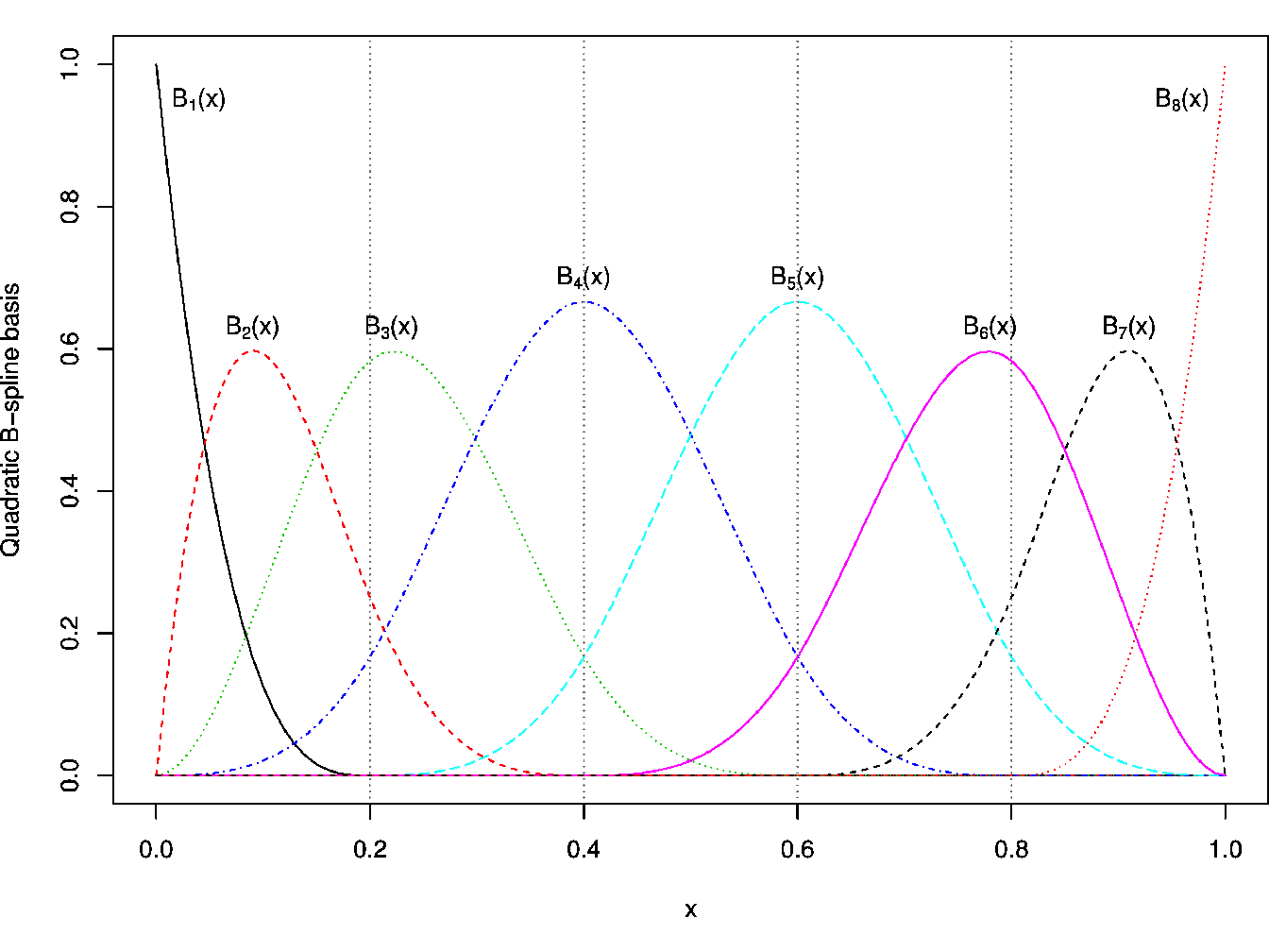
Figure 2.4: Quadratic \(\mathrm{B}\)-spline basis function representation (for \(m = 2\) and with \(K=4\) internal knots). Each \(B_k(\boldsymbol{x})\) functions are piecewise cubic and \(K+4 = 8\) of them are need to span the entire space.

2.4.4 Cubic smoothing splines

This smoother is constructed as the solution to an optimization problem: among all function \(f(x)\) with two continuous derivatives, find one that minimizes the penalized residual sum of squares

\[\sum_{i=1}^n||y_i - s(x_i)||_2^2 + \lambda \int_a^b{s''(t)}^2dt, \label{eq:cubsmooth}\]

where \(\lambda\) is a penalty factor, and \(a \leq x_1 \leq \dots \leq x_n \leq b\). The first term measures closeness to the data while the second penalizes curvature in the function, this criterion insuring a trade-off between bias and variance. The first term insures to fit as close as possible the data while the second penalizes the wiggliness of the smoothing curve to avoid interpolating the data. Large values of \(\lambda\) produce smoother curves while smaller values produce more wiggly curves.

As \(\lambda \rightarrow \infty\), the penalty term dominates, forcing \(s''(x) = 0\) everywhere and thus the solution is the least-squares line. On the contrary, as \(\lambda \rightarrow 0\), the penalty term becomes unimportant and the solution tends to an interpolating twice-differentiable function.

Furthermore, it can be shown that this optimization problem has an explicit, unique minimizer which proves to be a natural cubic spline with knots at the unique value of \(x_i\) (see (Reinsch 1967)).

We consider the smoothing function in the form: \[s(x) = \sum_{k=1}^{K} N_k(x) \beta_k, \label{eq:smooth_fun}\] where the \(N_k(x)\) are an \((K)\)-dimensional set of basis functions for representing the family of natural splines. The natural cubic splines basis is computed as follow: \[\begin{aligned} N_1(x) &= 1,\\ N_2(x) & = x, \\ N_{k+2}(x) &= d_k(x) - d_{k-1}(x), \end{aligned}\] for \(k \in [0, \dots, K-1]\) and with

\[d_k = \frac{(x-\xi_k)^3_+ - (x-\xi_K)^3_+}{\xi_K - \xi_k}\]

At first glance it would seems that the model is over-parametrized since there are as many as \(K = n\) knots implying as many degrees of freedom. However, the penalty term converts into a penalty on the splines coefficients themselves, which are shrunk toward the linear fit.

Using this cubic spline basis for \(s(x)\) means that can be written in the following minimization problem: \[\begin{equation} \underset{\boldsymbol{\beta}}{\text{argmin}} ||\mathbf{y} - \mathbf{N} \boldsymbol{\beta}||^2 + \lambda \boldsymbol{\beta}^T \mathbf{W} \boldsymbol{\beta} \tag{2.2} \end{equation}\] where \[\begin{aligned} N_{ik} &= N_k(x_i), \\ W_{kk'} &= \int_0^1 N''_k(x) N''_{k'}(x)dx,\end{aligned}\] with \(\mathbf{W} \in \mathbb{R}^{n \times n}\) the penalty matrix and \(\mathbf{} \in \mathbb{R}^{n \times n}\) the matrix of basis functions.

Following (Gu 2002), it can be shown that \[\begin{aligned} W_{i+2,i'+2} & = \frac{\left[\left(x_{i'} - \frac{1}{2}\right)^2 - \frac{1}{12}\right]\left[\left(x_{i} - \frac{1}{2}\right)^2 - \frac{1}{12}\right]}{4} - \\ & \frac{\left[\left(|x_{i} -x_{i'}| - \frac{1}{2}\right)^4 - \frac{1}{2}\left(|x_{i}-x_{i'} | - \frac{1}{2}\right)^2 + \frac{7}{240}\right]}{24},\end{aligned}\] for \(i,i' \in [1,\dots,K]\) with the first 2 rows and columns of \(\mathbf{W}\) are equal to \(0\). For a given \(\lambda\), the minimizer of , the penalized least squares estimator of \(\boldsymbol{\beta}\), is:

\[\hat{\boldsymbol{\beta}} = (\mathbf{N}^T\mathbf{N} + \lambda\mathbf{W})^{-1}\mathbf{N}^T\mathbf{y}.\]

It is interesting to note that this solution is similar to the ridge estimate , relating the smoothing splines to the shrinkage methods. Similarly the hat matrix, \(\mathbf{A}\), for the model can be written as

\[\mathbf{A} = \mathbf{N}(\mathbf{N}^T\mathbf{N} + \lambda\mathbf{W})^{-1}\mathbf{N}^T.\]

However, in spite of their apparent simplicity, these expressions are not the ones to use for computation. More computationally stable methods are preferred, i.e. the linear smoother described in (Buja, Hastie, and Tibshirani 1989), to estimate the smooth function \(s(x)\) (see Annexe @ref(#linsmooth) for more details). For the choice of the smoothing parameter \(\lambda\), see Annexe @ref(#lambda_smooth) and for an illustration of the cubic smoothing spline fit see Figure 2.5.

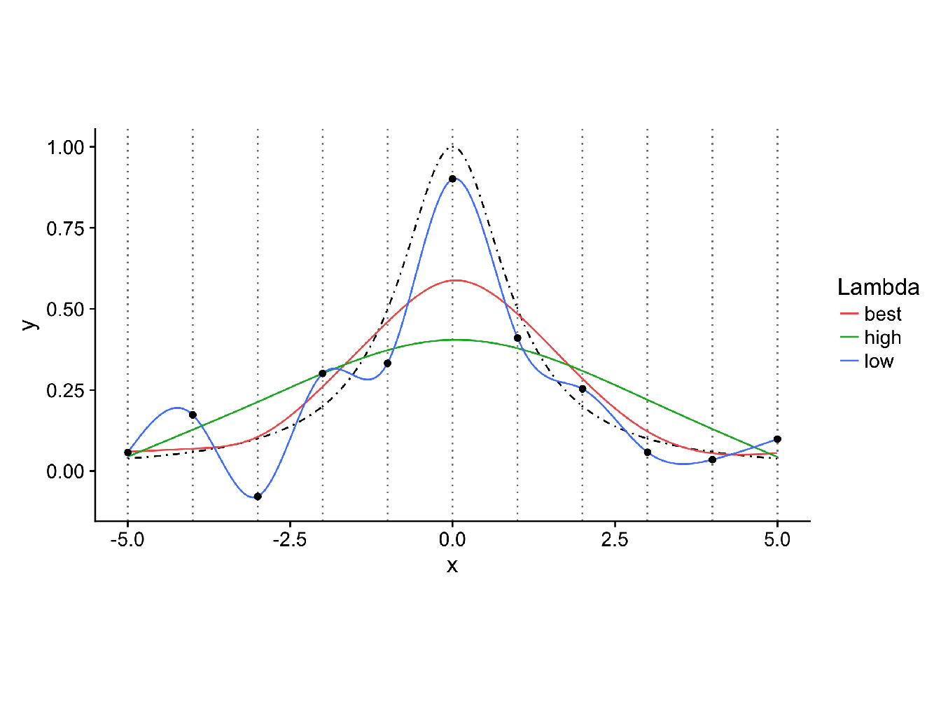
Figure 2.5: Cubic smoothing splines with different values of the regularization parameter \(\lambda\). The black dashed line corresponds to the true distribution \(y = \frac{1}{1+x^2}\) and each black dot corresponds to observations drawn from this distribution (with a little noise). In red is represented the fit at the best value of \(\lambda\) (chosen by GCV), in blue the fit with a value of lambda close to \(0\) and in green the fit with a high value for \(\lambda\). We can see that, as \(\lambda\) increase, the fit pass from a ’wiggly’ interpolating curve (as in Figure 2.5 to a very smoothed curve, which will eventually lead to a straight line as \(\lambda\) become very large.

2.4.5 Generalized additive models (GAM)

A generalized additive model (Hastie and Tibshirani 1990) is a generalized linear model with a linear predictor involving a sum of smooth functions of \(D\) covariates.

\[g(\theta) = \beta_0 + \sum_{d=1}^D s_d(\boldsymbol{x}_d) + \boldsymbol{\epsilon} , \label{eq:gam}\]

where \(\theta \equiv \mathbb{E}(\mathrm{Y} | \mathbf{X})\), \(\mathrm{Y}\) belongs to some exponential family distribution and \(g\) a known, monotonic, twice differentiable link function.

To estimate such model we can specify a set of basis functions for each smooth function \(s_d(x)\).

For instance, with natural cubic splines, we get the following model: \[g(\theta) = \beta_0 + \sum_{d=1}^D \sum_{k=1}^{K_d} \beta_{dk} N_{dk}(\boldsymbol{x}_d) + \boldsymbol{\epsilon} ,\] where \(K_d\) is the number of knots for variable \(d\).

Furthermore, if we use cubic smoothing splines for each smooth function \(s_d(x)\), we can define a penalized sum of squares problem of the form:

\[RSS(\beta_0, s_1, \dots, s_D) = \sum_{i=1}^n [y_i - \beta_0 - \sum_{d=1}^D s_d(x_{id})]^2 + \sum_{d=1}^D \lambda_d \int s''_d(t_d)^2dt_d.\]

Each smoothing spline function \(s_d(\boldsymbol{x})\) are then computed as described in Section 2.4.4 and the general model can be fitted with several methods such as backfitting or P-IRLS (Penalized-Iteratively Reweighted Least Squares) (Hastie and Tibshirani 1990).

Fitting GAMs by backfitting

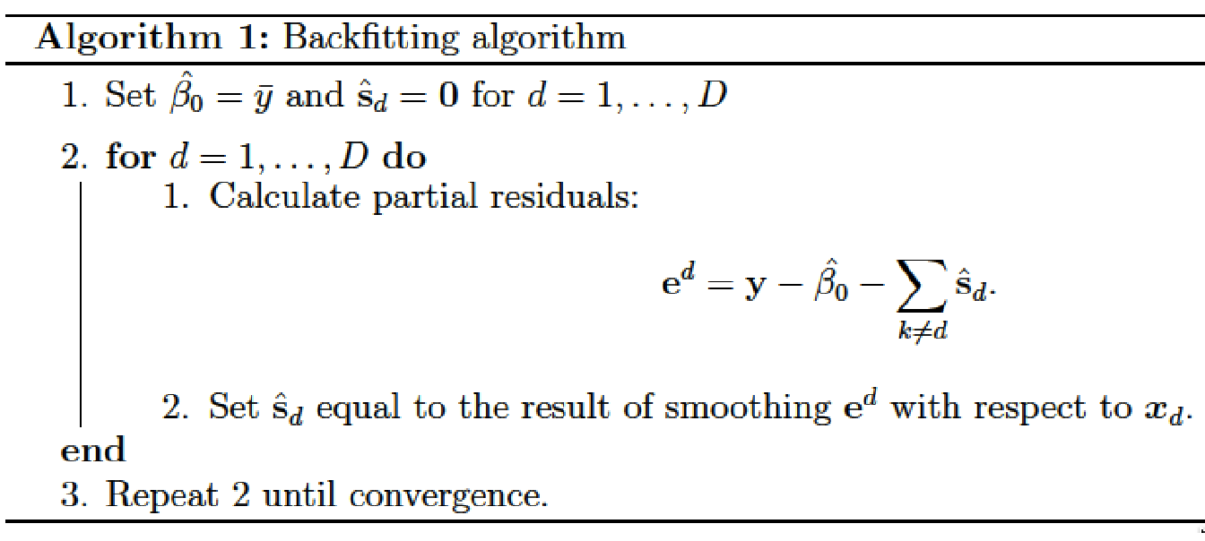
Backfitting is a simple procedure to fit generalized additive models which allow to use a large range of smooth function to represent the non-linear part of the model. Each smooth component is estimate by iteratively smoothing partial residuals from the additive model, with respect to the covariates that the smooth relates to. The partial residuals relating to the \(d^{th}\) smooth term are the residuals resulting from subtracting all the current model term estimates from the response variable except for the estimate of \(d^{th}\) smooth.

Given the following additive model: \[\mathbf{y} = \beta_0 + \sum_{d=1}^D s_d(\boldsymbol{x}_d) + \boldsymbol{\epsilon}.\]

Let \(\hat{\mathbf{s}}_d\) denote the vector whose \(i^{th}\) element is the estimate of \(s_d(x_{id})\). The backfitting algorithm is given in Algorithm 1.

2.4.6 High-dimensional generalized additive models (HGAM)

We consider an additive regression models in an high-dimensional setting with a continuous response \(\mathbf{y} \in \mathbb{R}^n\) and \(D \gg n\) covariates \(\boldsymbol{x}_1, \dots, \boldsymbol{x}_D \in \mathbb{R}^D\) connected through the model

\[\mathbf{y} = \beta_0 + \sum_{d=1}^D s_d(\boldsymbol{x}_d) + \boldsymbol{\epsilon},\]

where \(\beta_0\) is the intercept term, \(\boldsymbol{\epsilon} \sim \mathcal{N}(0, \mathbf{I}\sigma^2)\) and \(s_d : \mathbb{R} \rightarrow \mathbb{R}\) are smooth univariate functions. For identification purposes, we assume that all \(s_d\) are centered to have zero mean.

Sparsity-smoothness penalty

In order to get sparse and sufficiently smooth function estimates, (Meier, Geer, and Buhlmann 2009), proposed the sparsity-smoothness penalty

\[J(s_d) = \lambda_1\sqrt{||s_d||^2_n + \lambda_2\int[s''_d(\boldsymbol{x}_d)]^2d\boldsymbol{x}}.\]

The two tuning parameters \(\lambda_1, \lambda_2 \geq 0\) control the amount of penalization. The estimator is given by the following penalized least squares problem:

\[\hat{s}_1,\dots,\hat{s}_D = \underset{s_1,\dots,s_D\in\mathcal{F}}{\text{argmin}} ||\mathbf{y} - \sum_{d=1}^D s_d||_n^2 + \sum_{d=1}^D J(s_d),\] where \(\mathcal{F}\) is a suitable class of functions and the same level of regularity for each function \(s_d\) is assumed.

Computational algorithm

For each functions \(s_d\) we can use a cubic \(\mathrm{B}\)-spline parametrization with \(K\) interior knots placed at the empirical quantile of \(\boldsymbol{x}_d\). \[s_d(\boldsymbol{x}) = \sum_{k=1}^K\beta_{dk}b_{dk}(\boldsymbol{x}_d),\] where \(b_{dk}(x)\) are the B-spline basis functions and \(\boldsymbol{\beta}_d = (\beta_{d1},\dots,\beta_{dK})^T \in \mathbb{R}^K\) is the parameter vector corresponding to \(s_d\).

For twice differentiable functions, the optimization problem can be reformulated as

\[\hat{\boldsymbol{\beta}} = \underset{\boldsymbol{\beta}=(\beta_1,\dots,\beta_D)}{\text{argmin}} ||\mathbf{y} - \mathbf{B}\boldsymbol{\beta}||_n^2 + \lambda_1 \sum_{d=1}^D \sqrt{\frac{1}{n} \boldsymbol{\beta}_d^T\mathbf{B}_d^T\mathbf{B}_d\boldsymbol{\beta}_d + \lambda_2 \boldsymbol{\beta}_d^T \mathbf{W}_d\boldsymbol{\beta}_d},\]

\[= \underset{\boldsymbol{\beta}=(\boldsymbol{\beta}_1,\dots,\boldsymbol{\beta}_D)}{\text{argmin}} ||\mathbf{y} - \mathbf{B} \boldsymbol{\beta}||_n^2 + \lambda_1 \sum_{d=1}^D \sqrt{\boldsymbol{\beta}_d^T \left( \frac{1}{n} \mathbf{B}_d^T \mathbf{B}_d + \lambda_2 \mathbf{W}_d \right) \boldsymbol{\beta}_d},\] where \(\mathbf{B} = [\mathbf{B}_1|\mathbf{B}_2|\dots|\mathbf{B}_D]\) with \(\mathbf{B}_d\) is the \(n \times K\) design matrix of the \(B\)-spline basis of the \(d^{th}\) predictor and where the \(K \times K\) matrix \(\mathbf{W}_d\) contains the inner products of the second derivative on the \(B\)-spline basis function.

The term \((1/n)\mathbf{B}_d^T \mathbf{B}_d + \lambda_2\mathbf{W}_j\) can be decomposed using the Choleski decomposition \[(1/n) \mathbf{B}_d^T\mathbf{B}_d + \lambda_2\mathbf{W}_d = \mathbf{R}_d^T \mathbf{R}_d\] to some quadratic \(K \times K\) matrix \(\mathbf{R}_d\) and by defining \[\tilde{\boldsymbol{\beta}}_d = \mathbf{R}_d \boldsymbol{\beta}_d \text{ and } \tilde{\mathbf{B}} = \mathbf{B}_d \mathbf{R}_d^{-1},\] the optimization problem reduces to

\[\hat{\tilde{\boldsymbol{\beta}}} = \underset{\boldsymbol{\beta}=(\boldsymbol{\beta}_1,\dots,\boldsymbol{\beta}_D)}{\text{argmin}} ||\mathbf{y} - \tilde{\mathbf{B}}\tilde{\boldsymbol{\beta}}||^2_n + \lambda_1\sum_{d=1}^D||\tilde{\boldsymbol{\beta}_d}||,\]

where \(||\tilde{\boldsymbol{\beta}}_d|| = \sqrt{K}||\tilde{\boldsymbol{\beta}}_d||_K\) is the Euclidean norm in \(\mathbb{R}^K\). This is an ordinary group lasso problem for any fixed \(\lambda_2\), and hence the existence of a solution is guaranteed. For \(\lambda_1\) large enough, some of the coefficient groups \(\beta_d \in \mathbb{R}^K\) will be estimated to be exactly zero. Hence, the corresponding function estimate will be zero. Moreover, there exists a value \(\lambda_{1,max} < \infty\) such that \(\hat{\tilde{\boldsymbol{\beta}}}_1 = \dots = \hat{\tilde{\boldsymbol{\beta}}}_D = 0\) for \(\lambda_1 \geqslant \lambda_{1,max}\). This is especially useful to construct a grid of \(\lambda_1\) candidate values for cross-validation (usually on the log-scale). By rewriting the original problem in this last form, already existing algorithms can be used to compute the estimator. Coordinate-wise approaches as in (Meier, Van De Geer, and Buhlmann 2008) and (Yuan and Lin 2006) are efficient and have rigorous convergence properties.

References

Boor, Carl de. 1975. A Practical Guide to Splines. Springer. Springer. http://www.springer.com/gb/book/9780387953663.

Buja, Andreas, Trevor Hastie, and Robert Tibshirani. 1989. “Linear Smoothers and Additive Models.” The Annals of Statistics 17 (2): 453–510. http://www.jstor.org/stable/2241560.

Gu, Chong. 2002. Smoothing Spline ANOVA Models. Springer Series in Statistics. New York, NY: Springer New York. http://link.springer.com/10.1007/978-1-4757-3683-0.

Hastie, T. J., and R. J. Tibshirani. 1990. Generalized Additive Models. CRC Press.

Meier, Lukas, Sara van de Geer, and Peter Buhlmann. 2009. “High-Dimensional Additive Modeling.” The Annals of Statistics 37: 3779–3821. https://doi.org/10.1214/09-AOS692.

Meier, Lukas, Sara Van De Geer, and Peter Buhlmann. 2008. “The Group Lasso for Logistic Regression.” Journal of the Royal Statistical Society: Series B (Statistical Methodology) 70 (1): 53–71. http://onlinelibrary.wiley.com/doi/10.1111/j.1467-9868.2007.00627.x/abstract.

Reinsch, Christian H. 1967. “Smoothing by Spline Functions.” Numer. Math. 10 (3): 177–83. http://dx.doi.org/10.1007/BF02162161.

Yuan, Ming, and Yi Lin. 2006. “Model Selection and Estimation in Regression with Grouped Variables.” JOURNAL OF THE ROYAL STATISTICAL SOCIETY, SERIES B 68: 49–67.