4.5 Generalized additive models in GWAS

So far, we have modelled the phenotype as a linear function of the predictors using the logistic linear regression framework but we could also be interested to put forward non-linear relationships. One way to achieve this would be to use smoothing splines and generalized additive models (Section 2.4.4 and 2.4.5). Implementation of such methods in classical GWAS is not straightforward because the predictors are ordinal variables which take at most three different values (\(\lbrace 0,1,2 \rbrace\) with additive coding), making the use of smoothing splines irrelevant. However, in our context where we average the values of the SNP in each group, the use of smoothing splines becomes appropriate and may lead to the identification of non-linear otherwise undetectable with classical linear regression framework. We can nevertheless qualify this statement by mentioning that the SKAT model may also be able to identify non-linear relationships with an appropriate choice of kernel function, e.g. the weighted quadratic kernel.

We chose to focus on smoothing splines rather than other functions because they are, in our opinion, more easily interpretable. More specifically we seek at first to investigate what benefit we could take from replacing the ridge regression model in Algorithm 4 by the high-dimensional additive models (HGAM) described in Section 2.4.6 to estimate the optimal number of groups. Secondly, we would like to highlight non-linear behaviour between groups of SNP and the phenotype by fitting cubic smoothing splines on each of the aggregated-SNP predictors constructed at best level in the hierarchy.

4.5.1 Comparison of predictive power

To evaluate the contribution of generalized additive models in our methodology, we compare the results in term of predictive power of four different regression model used to estimate an optimal number of clusters for the ankylosing spondylitis dataset. Specifically, we compare the AUC-ROC curves obtained from Algorithm 4 when using respectively lasso, group-lasso, HGAM and ridge regression as the learning method. The results are presented in Figure 4.11. Note that for the group-lasso, the algorithm was applied at the single-SNP level rather than the aggregated-SNP.

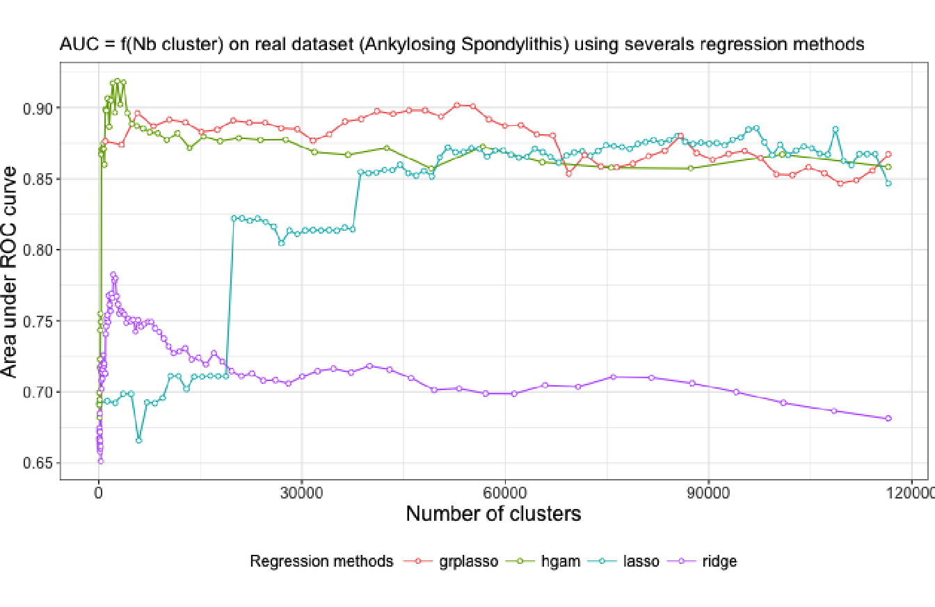
Figure 4.11: AUC-ROC plot illustrating the predictive power of four statistical learning approaches for several levels of a hierarchical clustering applied on the ankylosing spondylitis dataset.

We observe a similar pattern between the ridge regression curve and the HGAM curve, with about the same optimal number of clusters identified. The use of cubic smoothing splines in the model greatly increase the predictive power compare to the others regression model. The group-lasso regression has a good predictive performance but is outperform by HGAM when we fit the model on the aggregated-SNP predictors at the best cut-level.

4.5.2 Results of univariate smoothing splines on aggregated-SNP

4.5.2.1 Manhattan plot

The best cut-level identified using high-dimensional additive model is set to 2750 aggregated-SNP. Firstly, to each of these variables, a univariate additive model using cubic smoothing splines with knots at each unique value is fitted. Secondly, we calculate p-value for each smooth as described in Section 2.6.4. The results are shown in Figure 4.12, where 23 significant aggregated-SNP have been identified.

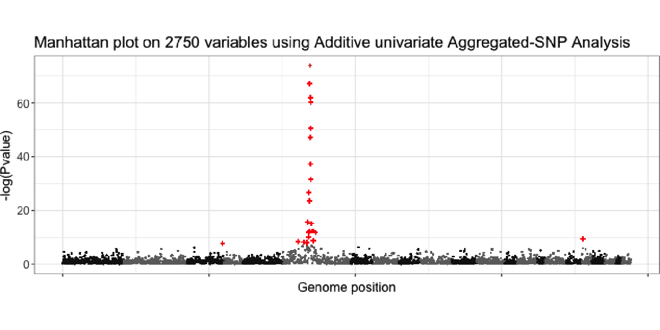
Figure 4.12: Manhattan plot of p-value calculated for 2750 aggregated-SNP using cubic smoothing splines.

4.5.2.2 Fitted values of the most significant aggregated-SNP

In this section, the plots in Figure 4.13 represent the fitted value of the 23 most significant aggregated-SNP variables previously identified. These aggregated-SNP are almost all located on the same region, on chromosome 6, region having already been identified as genetic risk factor for the disease (see Section 4.4.4. We only observe a new signal on chromosome 18 which could be interesting to investigate.

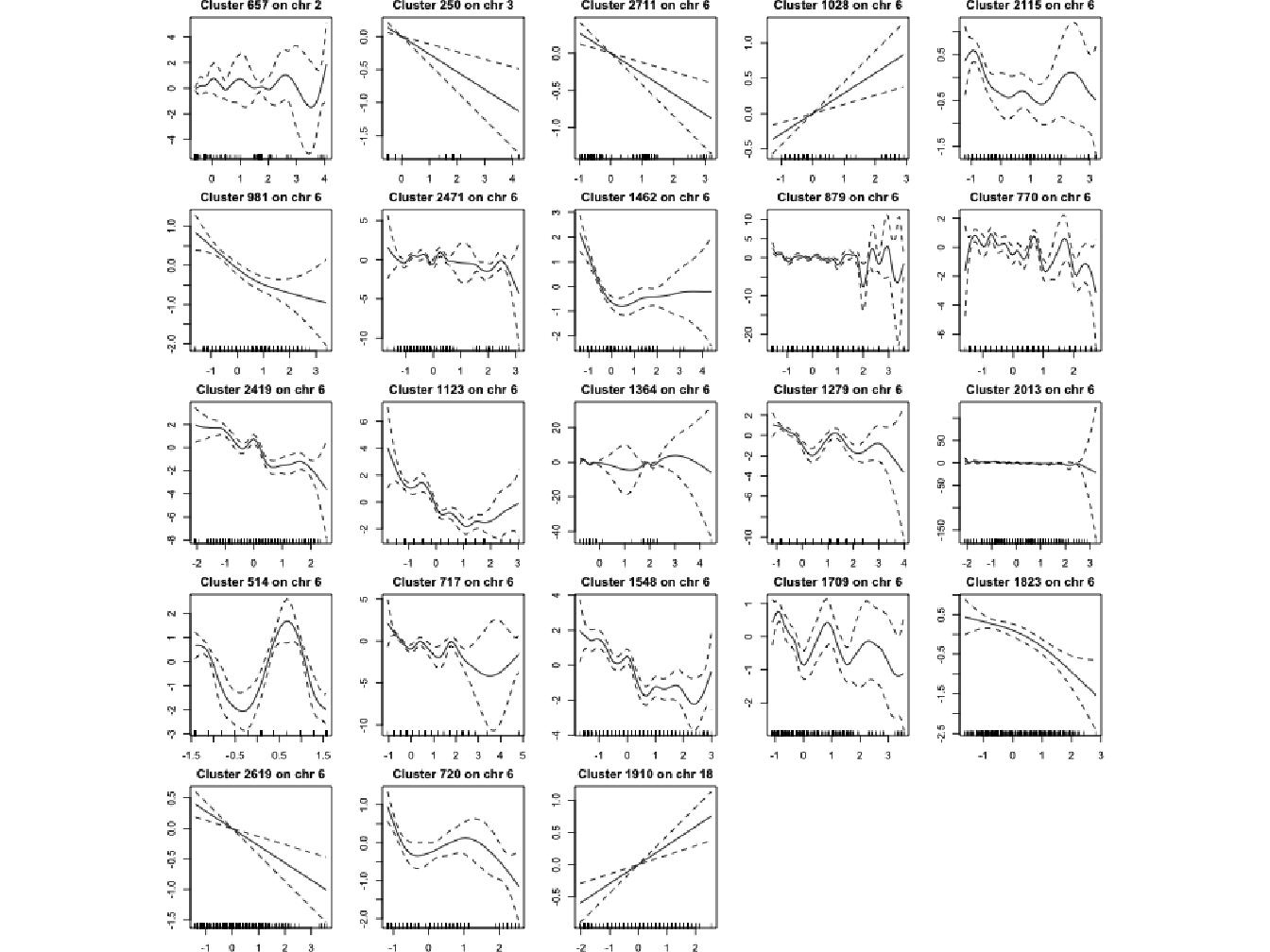
Figure 4.13: Representation of the smooth fits for the 23 most significant aggregated-SNP using cubic smoothing splines.

We observe that the significant regions identified on chromosome 6 have a non-linear behaviour. However, since these regions have also been identified with a classical linear regression approach, we cannot conclude that we have detected these regions thanks to the smoothing splines. Whether or not there is a non-linear behaviour, this region on chromosome 6 is always identified as associated with the disease. However, we could have thought that the new signal on chromosome 18 could be due to the non-linear nature of the association with the phenotype, but it is not the case. Indeed, if we look at the plot of the fitted value for this cluster, we can see that it is a straight line, leading to the conclusion that this signal might be a false positive.