3.2 Genotype quality control

In GWAS, the data filtering step used to identify genotyping mistakes is of primary importance since it can determine whether real discoveries are made or just false positives wrongly interpreted. With such large numbers of SNP being studied at the same time and with relatively moderate sample sizes, even small genotyping error rates can have a significant impact on the results.

As stated in (Wright and Hastie 2001), genetic effects on most multifactorial phenotypes follow an L-shaped distribution, with a few alleles having large effects and many alleles with a small effect size. This means that GWAS principally aim to identify small differences in allele frequencies between case and control, therefore even small experimental error can have strong effects on the results, particularly in the presence of rare alleles (Clayton et al. 2005; Barrett and Cardon 2006). The following paragraphs describe some of the filtering procedures designed to identify issues on specific SNP.

3.2.1 Deviation from HWE.

Neutral genetic variants in a large random-mating population are expected to display Hardy–Weinberg Equilibrium (see Section 1.5.1). However, observed frequencies might be modified by genotyping error, leading to a deviation from HWE. A traditional approach for detecting genotyping errors is to test such deviation using the Pearson goodness-of-fit statistic (Section 2.6.2 and to look for significant deviations from the HWE (Weir and Cockerham 1996). We usually perform this test only in the control sample since a deviation from HWE may also indicate an association with the disease. This test is insensitive to small deviations that are most often observed and, in a setting where there is a huge number of SNP to test for HWE deviation, an appropriate threshold of significance is therefore difficult to determine. Taking in account these considerations, the most prudent use of HWE tests for genotyping error may be only to exclude the most important deviations by setting an extreme significance threshold such as \(1.10^{-7}\) or less, and using exact tests for rare alleles (Weir et al. 2005).

3.2.2 Missing data.

In case-control studies, markers having large differences in missing data rates between cases and controls often yield false positives (Clayton et al. 2005). One can use the normal approximation to the binomial distribution to test for significant differences in missing data rates between cases and controls: \[z = \frac{m_c - m_t}{\sqrt{m(1-m)(1/n_0+1/n_1)}},\] with \(m_c\) and \(m_t\) the proportion of missing genotypes among cases and controls respectively, \(n_0\) and \(n_1\) the samples sizes of missing and non-missing data and \(m\) the overall missing genotype rate at the marker.

3.2.3 Distribution of test statistics.

When there are many significant loci coming out of a particular study it may more likely reflect systematic genotype error in some of those markers than reflect real discoveries. Indeed, remembering the L-shaped distribution of effect sizes, a study with \(10^5-10^6\) genetic markers genotyped on one or two thousand cases and equal numbers of controls should reveal few genuine loci with single locus p-values below \(1.10^{-6}\) (Zondervan and Cardon 2004). Quantile-Quantile plot (Q-Q plot) is an efficient graphical way to examine the distribution of p-value and to evaluate whether there are too many data points in the tail. Q-Q plots are constructed by ordering test statistics and plotting them against the corresponding ordered expected values (see Figure 3.1 for an example).

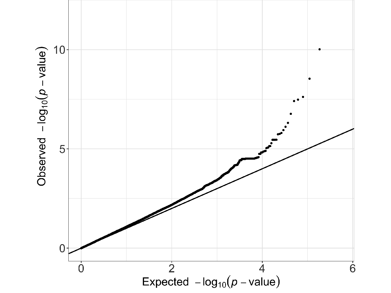
Figure 3.1: Example of Quantile-Quantile plot (Q-Q plot) representing the distribution of the test statistic for a classical GWAS study (results from GWAS analysis on Bipolar disorder data coming from the Welcome Trust Case-Control Consortium (WTCCC 2007)). In this example we can see that the smallest p-value is equal to \(4.5.10^{-5}\) and there are relatively few data points in the tail. Thus, based solely on the study of this distribution, there is therefore no reason to suspect genotyping errors.

References

Barrett, Jeffrey C, and Lon R Cardon. 2006. “Evaluating Coverage of Genome-Wide Association Studies.” Nature Genetics 38 (6): 659.

Clayton, David G, Neil M Walker, Deborah J Smyth, Rebecca Pask, Jason D Cooper, Lisa M Maier, Luc J Smink, et al. 2005. “Population Structure, Differential Bias and Genomic Control in a Large-Scale, Case-Control Association Study.” Nature Genetics 37 (11): 1243.

Weir, Bruce S, Lon R Cardon, Amy D Anderson, Dahlia M Nielsen, and William G Hill. 2005. “Measures of Human Population Structure Show Heterogeneity Among Genomic Regions.” Genome Research 15 (11): 1468–76.

Weir, Bruce S, and C Cockerham. 1996. “Genetic Data Analysis Ii: Methods for Discrete Population Genetic Data. Sinauer Assoc.” Inc., Sunderland, MA, USA.

Wright, Alan F, and Nicholas D Hastie. 2001. “Complex Genetic Diseases: Controversy over the Croesus Code.” Genome Biology 2 (8): comment2007–1.

WTCCC. 2007. “Genome-Wide Association Study of 14,000 Cases of Seven Common Diseases and 3,000 Shared Controls.” Nature 447 (7145): 661–78.

Zondervan, Krina T, and Lon R Cardon. 2004. “The Complex Interplay Among Factors That Influence Allelic Association.” Nature Reviews Genetics 5 (2): 89.